MMQGIS
Michael Minn (http://michaelminn.com)
14 February 2026
Describes use of MMQGIS, a set of Python vector map layer plugins for Quantum GIS
Introduction
MMQGIS is a set of Python plugins for manipulating vector map layers in Quantum GIS: CSV input/output/join, geocoding, geometry conversion, buffering, hub analysis, simplification, column modification, and simple animation. MMQGIS provides verbose progress reporting, an intuitive user interface, direct file access, and some additional capabilities missing from other plugin sets such as the Processing toolbox.
Getting MMQGIS
MMQGIS is included in the Quantum GIS Plugin Repository and should be readily available in the QGIS Python Plugin Installer (Plugins -> Fetch Python Plugins). A zip file of the current release is also available here for manual installation. Links to older versions are listed in the Version History at the bottom of this page.
Data Formats
Input layers can be from any geospatial data source supported by QGIS.
Output file format are implied by the file extension given on the output file name. Formats currently supported through OGR/GDAL include:
- ESRI Shapefile (*.shp)
- GeoJSON (*.geojson)
- SQLite (Spatialite) (*.sqlite)
- KML (*.kml)
- GPKG (GeoPackage SQLite file) (*.gpkg)
MMQGIS assumes that input and output files are encoded in the UTF-8 character set. MMQGIS uses the standard Python CSV file interface functions, which do not handle unicode or other multi-byte encodings. While files that use the lower 7-bits of the 8-bit Windoze character sets (ISO-8859-x) will generally be fine, unpredictable results and errors may occur with non-ASCII characters in non-UTF-8 character sets. See this and this for two ways to save a UTF-8 CSV from Excel.
Python Scripting with MMQGIS
MMQGIS contains a library module (mmqgis_library.py) that can also be used for Python scripting from the QGIS console, or in stand-alone scripts executed directly in Python. API information is included with the descriptions for each tool, and a guide to scripting is at the end of this document.
Licensing
MMQGIS is free software and is offered without guarantee or warranty. You can redistribute it and/or modify it under the terms of version 2 of the GNU General Public License (GPL v2) as published by the Free Software Foundation (www.gnu.org). Bug reports or suggestions are welcome at the e-mail address above, but I cannot promise a prompt or mutually satisfactory resolution.
Animation Tools
The animation tools create simple map animations as sequences of map image PNG files.
Images are exported from print layouts so at least one print layout must be defined. Map layouts permit adjustment of map extent, size, and DPI, as well as the ability to add additional cartographic elements to the output images.
Images may be combined into a single animated GIF using Gimp. This is the technique used for the example GIF files below.
Images may also be combine into video files using FFmpeg. For example, this creates a 30 FPS silent MPEG4 file using an h.264 codec that can be played in contemporary web browsers:
ffmpeg -r 30 -s 1280x720 -start_number 0 -i frames/frame%04d.png -vcodec libx264 -crf 1 -pix_fmt yuv420p temp.mp4
Animate Lines
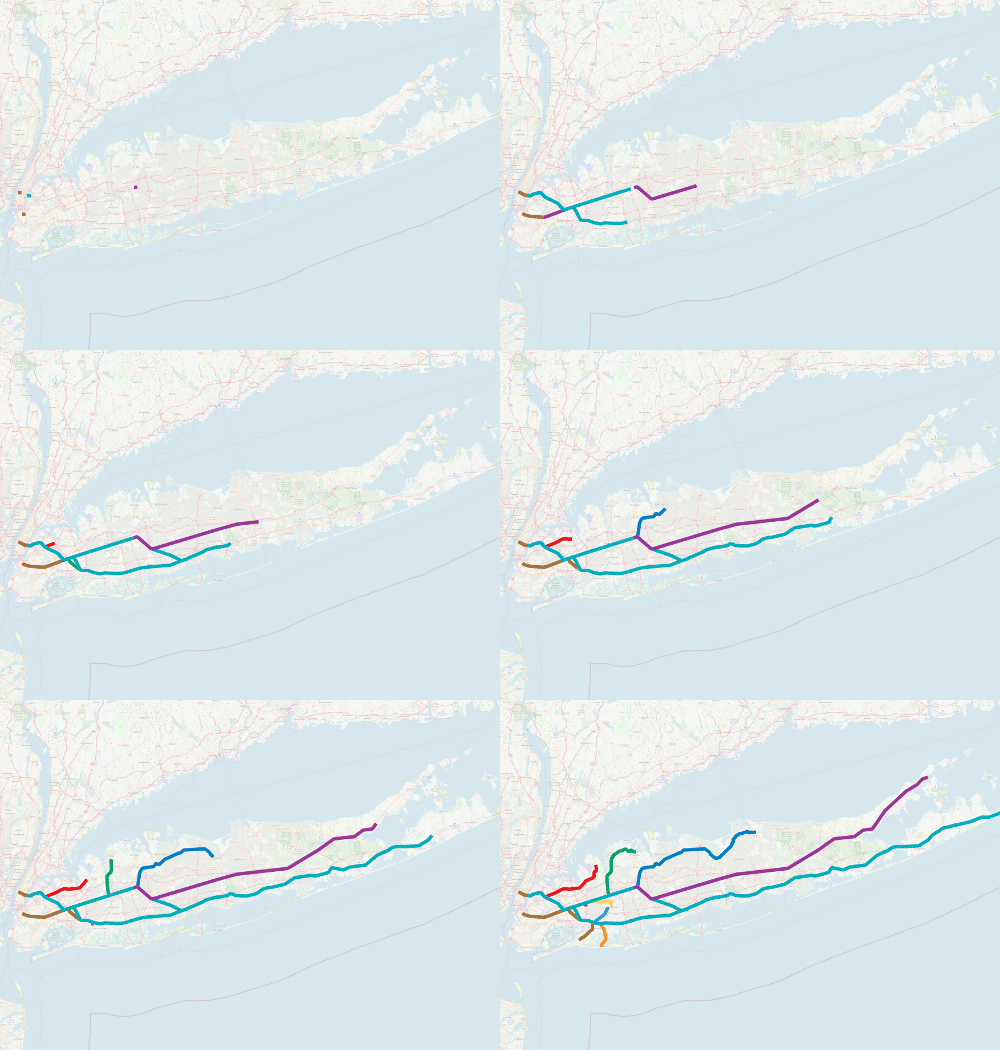
The Animate Lines tool creates animation of lines that grow to their full length over the duration of the animation. This is primarily useful as a visual effect.
The direction of growth is determined by the order of the linestring points in the source file. Depending on how the lines were digitized, this direction may be opposite of what is desired. To control the direction of growth, line vertices in the desired order can be created in a CSV file and imported with the Geometry Import From CSV File.
If attempting to animate a layer of MultiLineStrings, this tool will combine the points from all line segments into a single line of points. This will add spurious line segments to the animation if the points in the line segments were not ordered in a contiguous manner when digitized.
Parameters
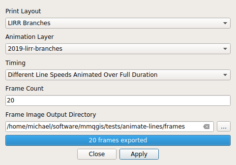
- Print Layout: The name of a print layout
- Animation Layer: The name of a linestring map layer that will be animated
- Timing:
- Different Line Speeds Animated Over Full Duration will grow all lines at different speeds so they all complete their full path simultaneously at the end of the animation
- One Line Speed Determined By Longest Line will grow all lines at the same linear speed, with the speed set by the longest line, which will complete at the end of the animation
- Frame Count: The number of separate frame files created
- Frame Image Output Directory: The directory where the frame PNG images will be saved
Python
mmqgis_animate_lines(print_layout, input_layer, fixed_speed, frame_count, \
			frame_directory, status_callback = None)
The example below animates branch lines of the Long Island Railroad in New York State.
- Line file: 2019-lirr-branches.geojson
- Project file: 2019-lirr-branches.qgs
# Paths to the project
test_directory = "/home/michael/software/mmqgis/tests/animate-lines"

# Remove any existing frames and create the frame directory
frame_directory = test_directory + "/frames"
shutil.rmtree(frame_directory, ignore_errors=True)
os.mkdir(frame_directory)

# Load the project
project_file = test_directory + "//2019-lirr-branches.qgs"
project = QgsProject.instance()
project.read(project_file)
if project.error():
	exit("Error: " + project.error())

# Find the parameters
print_layout = QgsProject.instance().layoutManager().printLayouts()[0]
layer = project.mapLayersByName("2019-lirr-branches")[0]
fixed_speed = True
frame_count = 20

# Run the tool and display any resulting error
message = mmqgis_animate_lines(print_layout, layer, fixed_speed, frame_count, frame_directory)
print("Animate lines: " + str(message))
Animate Location
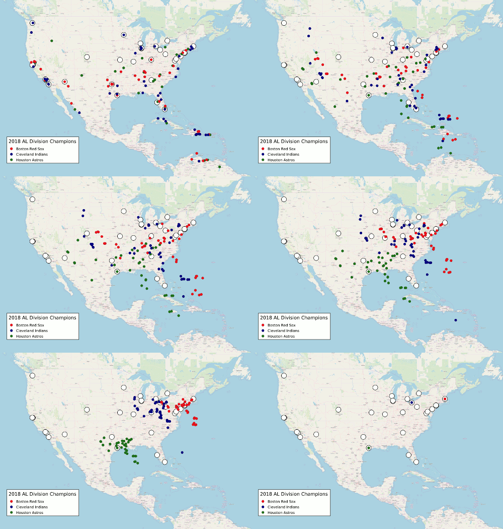
The Animate Location tool creates animations of map features as they move in a straight line to specified locations on separate destination map layer.
If you need more control over paths, you should use the Animate Sequence tool, or Anita Graser's TimeManager plugin.
This tool can be slow and processing-intensive if animating a large number of features.
Parameters
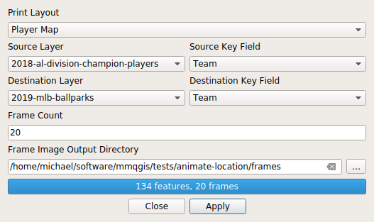
- Print Layout: The name of a print layout
- Source Layer: The name of the layer containing the features at their starting locations
- Source Key Field: The field in the source layer identifying the destination for each feature
- Destination Layer: The name of the layer containing locations where the source features will move to
- Destination Key Field: The name of the field in the destination layer identifying the destinations
- Frame Count: The number of separate frame files created
- Frame Image Output Directory: The directory where the frame PNG images will be saved
Python
mmqgis_animate_location(print_layout, source_layer, source_key_field, \
		destination_layer, destination_key_field, frame_count, \
		frame_directory, status_callback = None)
The example below animates the movement of the 134 players on the rosters of the three Major League Baseball teams that won the three divisions of the American League in 2019 from their birthplaces to the cities where their championship teams play. Data from BaseballAlmanac.com and Baseball-Reference.com. Geocoded with Nominatim. Ballpark data from Wikipedia.
- Player data: 2018-al-division-champion-players.geojson
- Ballpark data: 2019-mlb-ballparks.geojson
- Project file: 2018-al-division-champion-players.qgs
test_directory = "/home/michael/software/mmqgis/tests/animate-location"

# Load the project
# This needs to be a full path, otherwise layers do not get read in
project_file = test_directory + "/2018-al-division-champion-players.qgs"
project = QgsProject.instance()
project.read(project_file)
if project.error():
	exit("Error: " + project.error())

# Create the frame directory
frame_directory = test_directory + "/frames"
shutil.rmtree(frame_directory, ignore_errors=True)
os.mkdir(frame_directory)

# Parameters
print_layout = QgsProject.instance().layoutManager().printLayouts()[0]
source_layer = project.mapLayersByName("2018-al-division-champion-players")[0]
source_key_field = "Team"
destination_layer = project.mapLayersByName("2019-mlb-ballparks")[0]
destination_key_field = "Team"
frame_count = 10

# Run the function and print any error message
message = mmqgis_animate_location(print_layout, source_layer, source_key_field, \
		destination_layer, destination_key_field, frame_count, frame_directory)

print("Animate Location: " + str(message))
Animate Sequence
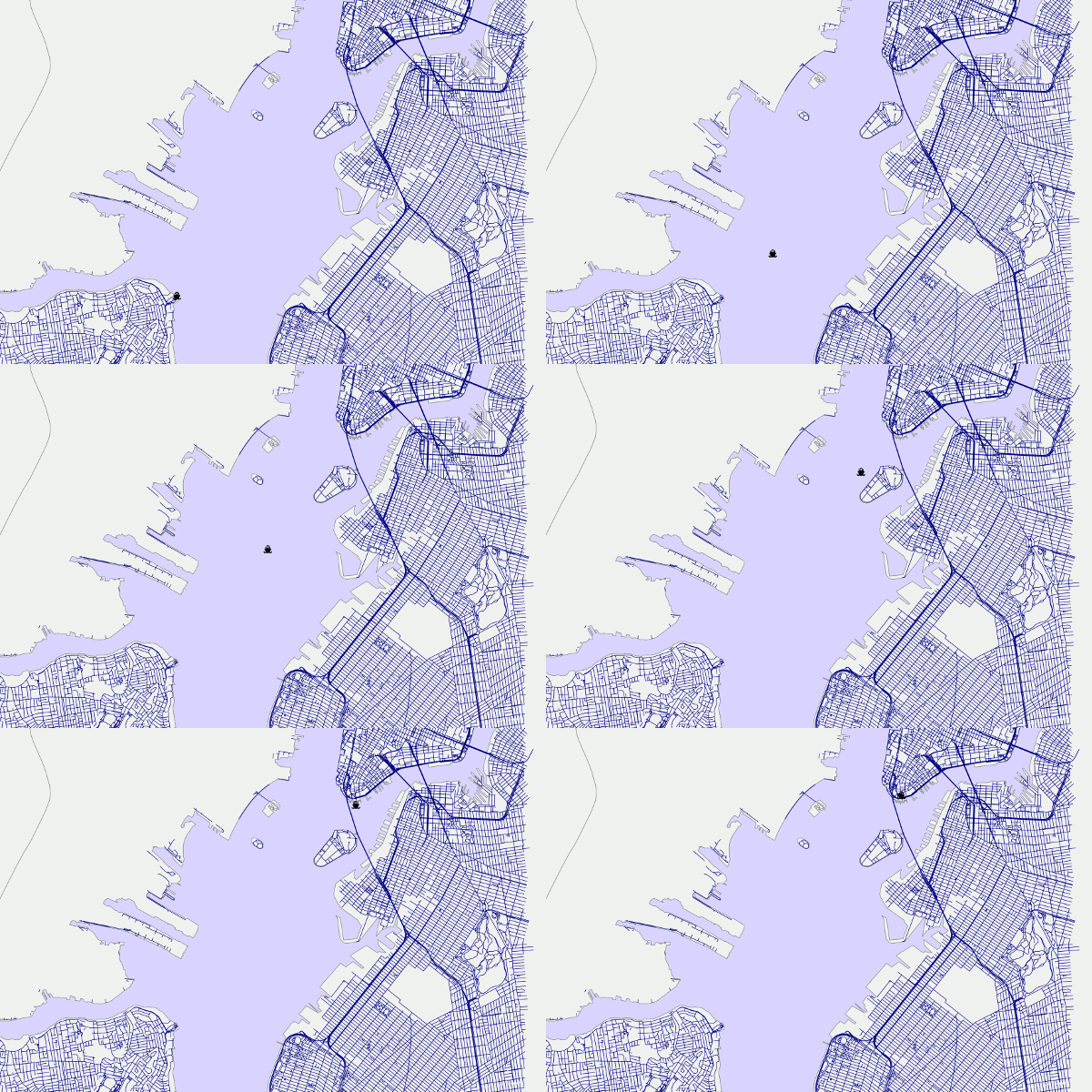
The Animate Sequence tool creates animations of map features in one or more layers by plotting successive rows in each layer.
If multiple layers are being animated simultaneously, the timing of rows in each layer will be the same. There is no capability for interpolating, frame skipping or frame duplication between layers of dissimilar length. If there are fewer rows in one animated layer than in another animated layer, no features from the shorter layer will be displayed after all rows in the shorter layer have been displayed.
Animate Sequence uses an edit buffer to sequentially display individual feature geometries. Therefore animated layers must be editable. If you wish to animate a non-editable layer (such as GPS waypoints from a GPX or CSV file), you should save the layer to an editable source, such as a shapefile, and animate the editable layer.
If text display of timing is desired, a layer must be created with a column that has the desired display text, and that layer must be mapped with features labeled.
If you need fine-grained control by specific times or a less cumbersome way of displaying current time, you may want to consider using Anita Graser's TimeManager plugin.
Parameters
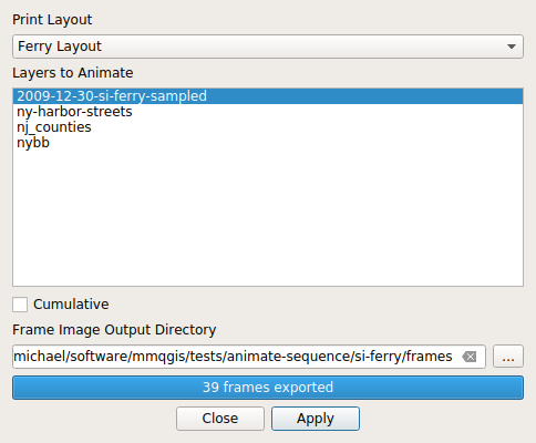
- Print Layout: The name of a print layout
- Layers to Animate: The name(s) of the layer(s) that will be animated
- Cumulative: If selected, previously plotted features will remain on the map. If not selected, only one feature per layer is displayed
- Frame Image Output Directory: The directory where the frame PNG images will be saved
Python
mmqgis_animate_sequence(print_layout, layers, cumulative, frame_directory, status_callback = None)
The example below animates sampled GPS waypoints tracking a trip on the Staten Island Ferry from St. George to South Ferry on 30 December 2009.
- Point data: 2009-12-30-si-ferry-sampled.geojson
test_directory = "/home/michael/software/mmqgis/tests/animate-rows/si-ferry"

# Load the project file
project_file = test_directory + "/animate-sequence.qgs"
project = QgsProject.instance()
project.read(project_file)
if project.error():
	exit("Error: " + project.error())

# Create the frame directory
frame_directory = test_directory + "/frames"
shutil.rmtree(frame_directory, ignore_errors=True)
os.mkdir(frame_directory)

# Parameters
print_layout = QgsProject.instance().layoutManager().printLayouts()[0]
layers = project.mapLayersByName("2009-12-30-si-ferry-sampled")
cumulative = False

# Run the tool
message = mmqgis_animate_sequence(print_layout, layers, cumulative, frame_directory)
print("Animate Sequence: " + str(message))
Animate Zoom
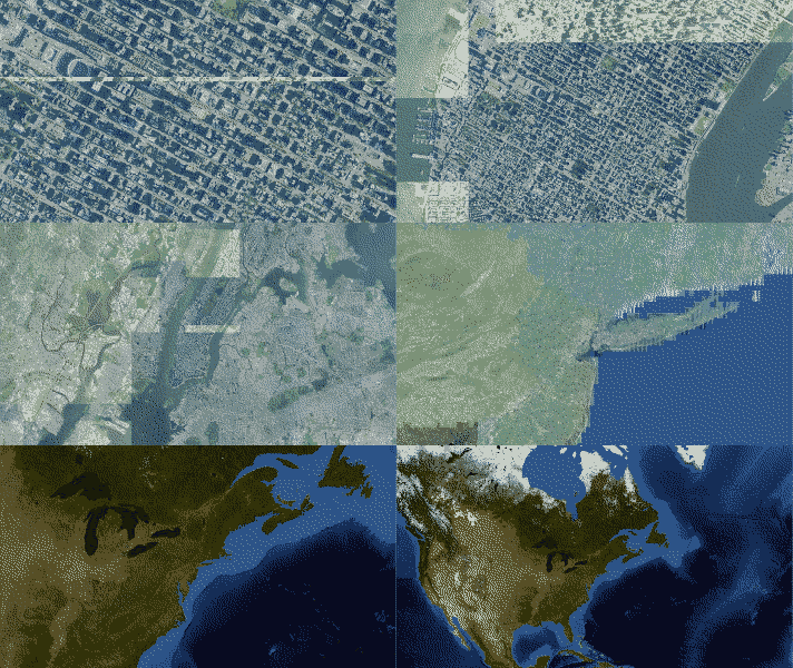
The Animate Zoom tool creates animations by zooming and or panning. This tool is especially useful for simulating motion across a landscape or zooming out to give context to a location.
Parameters
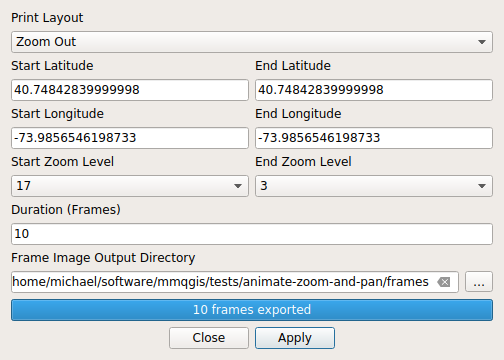
- Print Layout: The name of a print layout containing map items to animate. If the map contains multiple map items (such as with key maps), all map items will be animated
- Start Latitude / Longitude: The starting center location for the animation
- End Latitude / Longitude: The ending center location for the animation
- Start / End Zoom Level: Zoom levels are similar to the zoom levels for web maps, except the zoom level indicates the height of degrees of the map in latitude based on the formula: 360 / 2zoom_level. Zoom level one is pole to pole, while zoom level 10 usually covers a medium-sized city, and zoom level 20 is building level.
- Frame Count: The number of separate frame files created
- Frame Image Output Directory: The directory where the animation frame PNG images will be saved
Python
mmqgis_animate_zoom(print_layout, start_lat, start_long, start_zoom, \
		    end_lat, end_long, end_zoom, duration_frames, \
		    frame_directory, status_callback = None)
The example animates a zoom out on the USGS National Map ImageryOnly Base Map from NYC's Empire State Building to a whole-country view. Note that the USGS servers can be slow, so this script will take a few minutes to run even with a fairly small number of frames.
# US National Map: USGS ImageryOnly Base Map - Primary Tile Cache
# https://viewer.nationalmap.gov/services/
map_url = "crs=EPSG:3857&dpiMode=7&format=image/png&layers=0&styles&" + \
	"url=https://basemap.nationalmap.gov/arcgis/services/USGSImageryOnly/MapServer/WMSServer"
map_layer = QgsRasterLayer(map_url, "US National Map Imagery", 'wms')

# Create the print layout with a single page for a 1280x720 image at 300 DPI
print_layout = QgsPrintLayout(QgsProject.instance())
print_layout.initializeDefaults()
page_size = QgsLayoutSize(108.4, 61, QgsUnitTypes.LayoutMillimeters);
print_layout.pageCollection().page(0).setPageSize(page_size)

# Create a map item covering the whole page
map_item = QgsLayoutItemMap(print_layout)
map_item.setFixedSize(page_size)
map_item.attemptMove(QgsLayoutPoint(0, 0))
map_item.setCrs(map_layer.crs())
map_item.setExtent(QgsRectangle(-100000, -100000, 100000, 100000)) # arbitrary = tool changes this
map_item.setBackgroundColor(QColor("#2a578e")) # Ocean blue
map_item.setBackgroundEnabled(1)
map_item.setLayers([ map_layer ])

# Add the item to the layout
print_layout.addLayoutItem(map_item)

# Parameters
start_lat = 40.748481
start_long = -73.985707
start_zoom = 15
end_lat = 40.748481
end_long = -73.985707
end_zoom = 3
frame_count = 20
frame_directory = "/home/michael/software/mmqgis/tests/animate-zoom/frames"

message = mmqgis_animate_zoom(print_layout, start_lat, start_long, \
	start_zoom, end_lat, end_long, end_zoom, frame_count, \
	frame_directory, status_callback)

print("Animate Zoom: " + str(message))
Combine Tools
Attribute Join from CSV File
The Join Attributes tool combines attributes from a CSV file with an existing vector layer by performing a join using a "key" field that is present both in the CSV file and in the attribute table of the map layer to which the data is being joined.
Because CSV files contain no reliable type data in the header, data is always imported from CSV files as text. Text columns can be converted to numeric (floating point) using the "Text to Float" tool.
CSV files must be encoded in the UTF-8 character set. Although other 8-bit encodings (like Windoze ISO-8859-x) will work if only ASCII characters are present, non-ASCII characters may cause unpredictable behavior.
This join is an SQL FULL OUTER JOIN. If there are multiple occurances of a key in the CSV or map layer, there will be multiple combinations of the data in the output shapefile.
QGIS has the ability to perform table joins as part of projects. If you only need joined data for a specific project and/or the underlying data changes periodically, you may prefer to use table joins. Right click on the layer and select Properties -> Joins.
Parameters
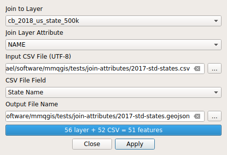
- Join to Layer: A vector layer of features to which the attributes will be attached
- Join to Attribute: The attribute in the vector layer that will be used as a key to match rows from the CSV file with features in the input layer
- Input CSV File (UTF-8): The name of the CSV file containing attributes that will be joined to the layer
- CSV File Field: The field in the CSV file that will be used as the key to match rows from the CSV file with features in the input layer
- Output File Name: The name of the output file that will contain the joined data
Python
mmqgis_attribute_join(input_layer, input_layer_attribute, \
		input_csv_name, input_csv_attribute, \
		output_file_name, status_callback = None)
The example below joins a USCB state cartographic boundary shapefile with 2017 CDC data on chlamdia, gonorrhea, and syphilis rates by state.
- State boundaries: cb_2018_us_state_500k.zip
- CSV data: 2017-std-states.csv
input_layer_name = "cb_2018_us_state_500k.shp"
input_layer = QgsVectorLayer(input_layer_name)
input_layer_attribute = "NAME"
input_csv_name = "2017-std-states.csv"
input_csv_attribute = "State Name"
output_file_name = "2017-std-states.geojson"

message = mmqgis_attribute_join(input_layer, input_layer_attribute,
		input_csv_name, input_csv_attribute, output_file_name)
print("Attribute Join: " + str(message))
Merge Layers
The Merge Layers tool merges features from multiple layers into a single shapefile and adds the merged shapefile to the project.
Merged layers must all be the same geometry type (point, polygon, etc.).
If the source layers have different attribute fields (distinguished by name and type), the merged file will contain a set of all different fields from the source layers with NULL values inserted when a source layer does not have a specific output field.
Where fields with the same name in different layers have different types, the output field type will be string.
Parameters
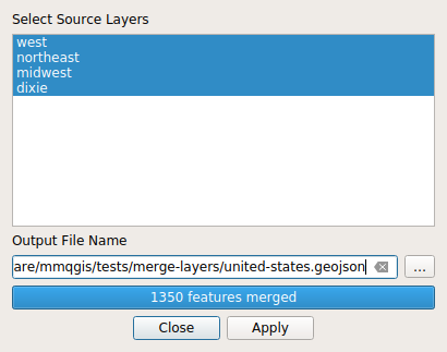
- Select Source Layers: The names of layers to merge
- Output File Name: The name of the output file that will contain the joined data
Python
mmqgis_merge(input_layers, output_file_name, status_callback = None)
The example below merges four regional data files into a single layer.
input_layer_1 = QgsVectorLayer("west.shp")
input_layer_2 = QgsVectorLayer("northeast.shp")
input_layer_3 = QgsVectorLayer("midwest.shp")
input_layer_4 = QgsVectorLayer("dixie.shp")
input_layers = [input_layer_1, input_layer_2, input_layer_3, input_layer_4]

output_file_name = "united-states.geojson"

message = mmqgis_merge(input_layers, output_file_name, status_callback)
print("Merge States: " + str(message))
Spatial Join
The Spatial Join tool combines attributes from different layers based on spatial relationship. The spatial joins are very common operations in standard GIS analysis.
A COUNT attribute is automatically appended to the output that indicates the number of related join layer features contributing data to each feature from the target layer.
Features from the target layer that have no spatial relationship to the join layer are not included in the output.
Parameters
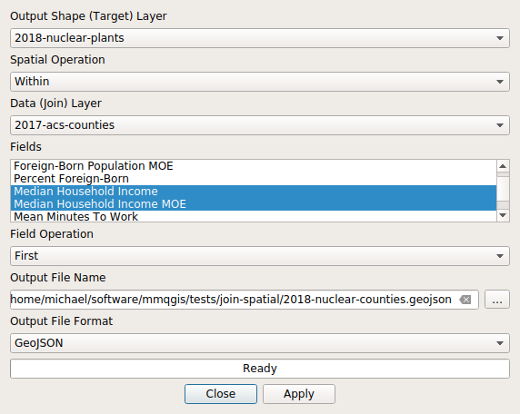
- Output Shape (Target) Layer: Indicates the layer that defines the shapes that will be the output by the tool
- Spatial Operation: Indicates the spatial relationship that should be used
in the operation. Some relationships are not available for some combinations of
shapes (ex: there is no within relationship when joining a polygon target layer
with a point join layer)
- Intersects: There is some intersection (overlap) between the target and join feature. This is probably the most common choice
- Within: The target feature is entirely within the join feature
- Contains: The join feature is entirely within the target feature
- Data (Join) Layer: Indicates the layer that will provide the data joined to the shape target layer specified above
- Field Operation: Indicates what should be done when multiple
features from the join layer have a relationship with the target layer:
- First: Takes the value of the first join feature encountered. This is dependent on the order of features in the underlying layer source and will be unpredictable unless you specifically know how the layer is organized. This is the default for fields that are not real numbers
- Sum: Takes the sum of values for all joined features
- Proportional Sum: Sums the data from each joined feature in proportion to the percentage of join feature area (in map units) covered by the target feature. Not meaningful for point target layers
- Average: Takes the average of values for all joined features
- Weighted Average: Takes the average of values for all joined features weighted in proportion to the percentage of target feature area (in map units) covered by the join feature. Not meaningful for point join layers
- Largest Proportion: Takes the value of the join feature that covers the largest proportion of area in the target feature
- Fields: Selection of the combined attributes from both source layers that will be included in the output. Multiple attributes can be selected. Selection capability is provided so that the output does not have to be cluttered with multiple unnecessary attributes
- Output File Name: The name of the output file that will contain the joined data
Python
mmqgis_spatial_join(target_layer, spatial_operation, join_layer, field_names, field_operation, \
	output_file_name, status_callback = None)
The example below joins nuclear reactor locations from Wikipedia and the NRC with county-level income data from the 2013-2017 American Community Survey to get the average median household income of counties containing nuclear reactors.
- Plant data: 2018-nuclear-plants.geojson
- County data: 2017-acs-counties.geojson
target_layer_name = "2018-nuclear-plants.geojson"
target_layer = QgsVectorLayer(target_layer_name)
spatial_operation = "Intersects"
join_layer_name = "2017-acs-counties.geojson"
join_layer = QgsVectorLayer(join_layer_name)
field_names = ["Median Household Income", "Median Household Income MOE", "Total Population", "County Name"]
field_operation = "First"
output_file_name = "2018-nuclear-counties.geojson"

message = mmqgis_spatial_join(target_layer, spatial_operation, join_layer, \
	field_names, field_operation, output_file_name, status_callback)
print("Spatial Join: " + str(message))

# Calculate average household income in nuclear counties weighted by population
moe = 0
income = 0
total_population = 0
output_layer = QgsVectorLayer(output_file_name)
for feature in output_layer.getFeatures():
	population = int(feature.attribute("Total Population"))
	moe = moe + (population * float(feature.attribute("Median Household Income MOE")))
	income = income + (population * float(feature.attribute("Median Household Income")))
	total_population = total_population + population

moe = moe / total_population
income = income / total_population
print("Nuclear counties: population " + str(total_population) + ", average income $" \
	+ str(income) + " +/- $" + str(moe))
Create Tools
Create Buffers
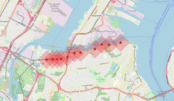
The Create Buffers tool creates polygon buffers around points, lines and polygons.
This tool expresses buffer sizes as absolute linear distance units (miles, feet, meters, kilometers defined by WGS 84 great circle distance) rather than map units. The haversine formula is used to approximate meaningful radius distances independent of the original projection. While this may introduce some deviation from the original CRS, buffering is assumed in practice to be an inexact operation that can usually tolerate such discrepancy.
Buffer radius can be fixed for all buffers as specified in the dialog, or buffer sizes can be taken from an attribute in the source shape layer.
Point buffers can be created with different numbers of edges: triangles, diamonds, pentagons, hexagons, 32-edge circles or 64-edge circles. If other numbers of edges, or different numbers of edges for different points are needed, the number of edges can be taken from a numeric attribute in the source shape layer.
Point buffers can be rotated based on a fixed number of degrees, or based on a numeric attribute in the source shape layer that indicates the rotation for each individual feature. The first node of a point buffer at zero degrees rotation is directly north from the point being buffered.
Line buffers can be created as normal rounded-end, single-sided, or flat-ended. Flat ended buffers are created by dissolving a north-sided and south-sided buffer for each line. This may cause odd shapes when line ends point in directions that deviate significantly from the general direction of the line. With multiple-line features, each line segment is treated as a separate shape, so angular deviations between line segments may result in slivers.
Line buffers can also be north-, south-, east- or west-side only. The determination of which side of the line is buffered is determined by the angular direction of line as defined by the start and end points of the line. This may result in undesirable results if buffering layers that mix vertically- and horizontally-oriented features. This tool does not currently have the capability to buffer based on directional characteristics like traffic or water flow through the features that lines are used to represent. For lines that are exactly perpendicular, the west side is considered the north side for north side buffering. For lines that are exactly horizontal, the south side is considered the west side.
Parameters
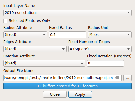
- Input Layer Name: The name of the map layer with features to create buffers around
- Selected Features Only: Buffer only selected features
- Radius Attribute: The name of the field in the input layer to use as the radius for each buffer. For a fixed radius, select "(fixed)"
- Fixed Radius: If no radius_attribute is given, use this fixed value for the radius
- Radius Unit: The distance unit for the radius. Options are "Meters" (the default), "Kilometers," "Feet," "Miles," or "Nautical Miles"
- Edges Attribute: The name of the field in the input layer to use for the number of edges on each buffer. For a fixed number of edges, select "(fixed)"
- Fixed Number of Edges: If no edge_attribute is given, use this as the number of edges (three or more)
- Rotation Attribute: The name of the field in the input layer to use as the rotation (in degrees) for each buffer. For a fixed rotation, select "(fixed)"
- Fixed Rotation (Degrees): If no rotation_attribute is given, use this fixed rotation (in degrees)
- Output File Name: The name of the output file that will contain the buffers
Python
mmqgis_buffers(input_layer, selected_only, radius_attribute, radius, radius_unit, \
	edge_attribute, edge_count, rotation_attribute, rotation_degrees, \
	output_file_name, status_callback = None)
The example below creates half-mile buffers around the stations on the abandoned North Shore Branch of the Staten Island Railway. Passenger service terminated on this line in 1953, and freight service terminated in 1989, although there is interest in reactivating the line as light rail or bus rapid transit.
- Point data: 2010-nsrr-stations.geojson
input_file_name = "2010-nsrr-stations.geojson"
input_layer = QgsVectorLayer(input_file)
selected_only = False
radius_attribute = None
radius = 0.5
radius_unit = "Miles"
edge_attribute = None
edge_count = 4
rotation_attribute = None
rotation_degrees = 0
output_file_name = "2010-nsrr-buffers.geojson"

message = mmqgis_buffers(input_layer, selected_only, radius_attribute, radius, radius_unit, \
	edge_attribute, edge_count, rotation_attribute, rotation_degrees, output_file_name)

print("Point Buffers: " + str(message))
Create Grid Layer
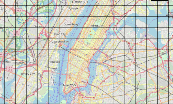
The Grid tool creates a layer containing a grid of shapes.
Parameters
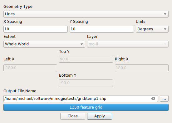
- Geometry Type:
- Lines: Creates separate horizontal and vertical lines for each grid cell
- Rectangles: Creates separate rectangles for each grid cell
- Points: Creates points at each grid cell corner
- Random Points: Creates points for each grid cell, with each point randomly located in each grid cell. This is useful for creating distributions of points that are random but have a known average spatial regularity
- Diamonds: Creates interlocking diamonds (rectangles rotated 45 degrees)
- Hexagon: Creates a grid of interlocking hexagons. To maintain equilaterality, the ratio between the horizontal and vertical spacing is fixed (and different). Changing horizontal spacing will automatically change vertical spacing, and vice versa.
- Extent: The grid extent can be automatically calculated from the current map window, the extent of a map layer, or the entire world, or it can be specified with user-defined values
- X Spacing: The distance between vertical lines
- Y Spacing: The distance between horizonatal lines
- Units: The unit to use for spacing distances. The units can be can be in degrees (WGS 84), the units of the coordinate reference system used by the project (Project Units), or the units for one of the map layers (Layer Units). Because many map projections distort distance, if you need a grid based on ground distance units (such as meters or feet), you should either define the project with a projected coordinate system or include a layer that has a projected coordinate system in the desired units
- Output File Name: The name of the output file for the grid
Python
mmqgis_grid(geometry_type, crs, x_spacing, y_spacing, \
	x_left, y_bottom, x_right, y_top, \
	output_file_name, status_callback = None)
The example below creates a ten-degree WGS 84 grid for the whole earth.
geometry_type = "Lines"
crs = QgsCoordinateReferenceSystem("PROJ4:+proj=longlat +datum=WGS84 +no_defs")
x_spacing = 10
y_spacing = 10
x_left = -170
x_right = 170
y_bottom = -80
y_top = 80
output_file_name = "world-grid.geojson"

message = mmqgis_grid(geometry_type, crs, x_spacing, y_spacing, \
	x_left, y_bottom, x_right, y_top, output_file_name)

print("Create Grid: " + str(message))
Hub Lines / Distance
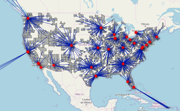
The Hub Lines / Distance tool creates spoke lines from spoke end points to hub points. Such layers are useful for visualizing catchment or distribution areas, or estimating travel distance.
The hub lines added to the output file with all attributes from the associated spoke points.
This tool does not incorporate any kind of network analysis, so if real-life paths to hubs are non-linear (e.g. when dealing with city blocks and other types of transportation networks), the closest great-circle or Euclidean distance may not be the closed in terms of traveling distance.
Parameters
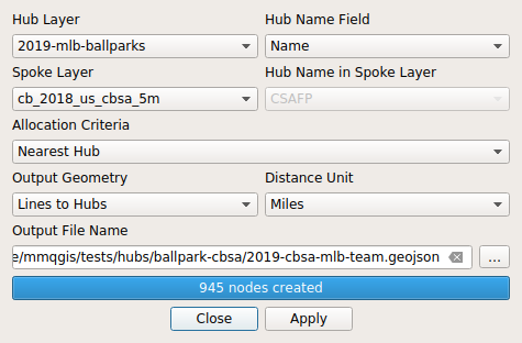
- Hub Layer: The name of the layer used for hub points
- Hub Name Field: The field in the hub layer used as the name for the hub
- Spoke Layer: The name of the layer used for spoke end points
- Hub Name in Spoke Layer: The field name in the hub layer giving the hub associated with each spoke. Only valid when the allocation criteria is Hub Name in Spoke Layer
- Allocation Criteria: The method in which hubs are assigned to spokes
- Nearest Hub: The nearest hub is used
- Hub Name in Spoke layer: The Hub Name Field in the hub layer is matched to the Hub Name in Spoke Layer field in the spoke end point layer
- Evenly Distribute: Spokes are evenly distributed to the nearest possible hubs. This algorithm sequentially assigns points to hubs, and then iterates through pairs of points while exchanging hubs when the combined point/hub distance of the pair would be smaller. This yields a graph with evenly distributed points and a minimized total point/hub distance. The minimization algorithm requires multiple passes and may be slow on large data sets. The minimized results should be mathematically valid, but may yield non-intuitive results depending on the spatial distribution of your data
- Output Geometry
- Lines to Hubs: The output features are lines connecting hubs to spoke end points
- Points: The output features are the spoke points with an added distance field
- Distance Unit: The distance unit used for the Distance field added to the output layer
giving the distance from the hub to the spoke end point
- If Layer Units is selected, Euclidean distance is calculated in the coordinate system used for the two layers. No attempt is made to transform between coordinate systems, and using source and hub layers with different coordinate systems may yield odd and undesirable results
- If Layer Units is not selected, points are converted to WGS84 and great-circle distances are calculated using the Haversine formula with Lambert's (1942) formula to correct for ellipsoidal flattening. Distance is then added as an attribute to the output file
- If your data is not WGS84 lat/long, it may be preferable to use Layer Units so the calculated distances are compatible with the distortions in your layer projection
- Output File Name: The name of the output feature file
Python
mmqgis_hub_lines(hub_layer, hub_name_field, spoke_layer, spoke_hub_name_field, \
	allocation_criteria, distance_unit, output_geometry, \
	output_file_name, status_callback = None)
The following example creates hubs between the centroids of major core-based statistical areas (metropolitan areas) and major league baseball parks to estimate geographic allegiance to MLB teams.
- CBSA data: cb_2018_us_cbsa_5m.shp
- Ballpark data: 2019-mlb-ballparks.geojson
hub_layer_name = "2019-mlb-ballparks.geojson"
hub_layer = QgsVectorLayer(hub_layer_name)
hub_name_field = "Team"
spoke_layer_name = "cb_2018_us_cbsa_5m.shp"
spoke_layer = QgsVectorLayer(spoke_layer_name)
spoke_name_field = "Name"
allocation_criteria = "Nearest Hub"
distance_unit = "Miles"
output_geometry = "Lines to Hubs"
output_file_name = "2019-cbsa-mlb-team.geojson"

message = mmqgis_hub_lines(hub_layer, hub_name_field, spoke_layer, spoke_name_field, \
	allocation_criteria, distance_unit, output_geometry, output_file_name)
print("Nearest Hubs: " + str(message))
Voronoi Diagram
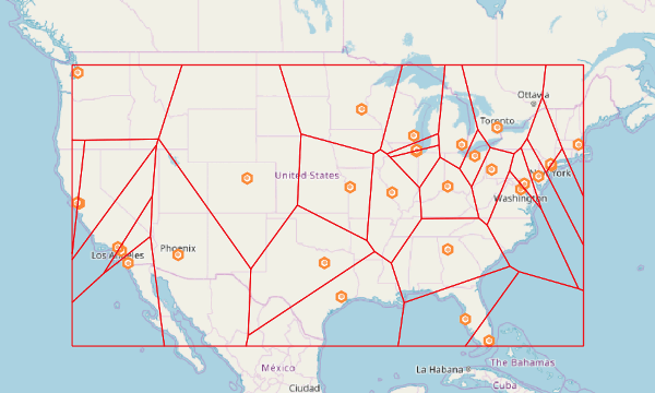
The Voronoi Diagram tool creates Voronoi diagrams, which are collections of polygons, each surrounding individual points and representing the area around each point that is closer to that point than any other. The shapes are named after Russian mathematician Georgy Fedoseevich Voronoi (1868-1908), who published a formal definition in 1908, but the concept of this type of polygon extends back to Descartes in the 17th century. Similar polygons were famously used by physician John Snow to trace the source of a London cholera epidemic in 1854 and Voronoi diagrams remain useful in GIS for analyzing areas of influence associated with individual points within a collection. Voronoi diagrams are also called Thiessen polygons, named after their usage in meteorology by Alfred Thiessen.
This tool requires an input point layer and outputs a polygon layer.
The boundary of the Voronoi diagram is the min/max extent of the points in the source layer.
The algorithm used to calculate the edges and nodes starts with tangents at the midpoints of lines between each point. The closest tangent is assumed to be a border and intersections to the border are calculated to circle each border until back to the beginning. The algorithm is computationally intensive, but still seems to run fairly quickly on a reasonably small set of points.
Parameters
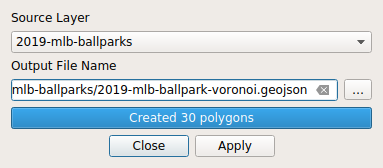
- Source Layer: The layer of points to build Voronoi polygons around
- Output File Name: The name of the output feature file
Python
mmqgis_voronoi_diagram(input_layer, output_file_name, status_callback = None)
The following example creates Voronoi polygons around major league baseball parks.
- Ballpark data: 2019-mlb-ballparks.geojson
input_layer_name = "2019-mlb-ballparks.geojson"
input_layer = QgsVectorLayer(input_layer_name)
output_file_name = "2019-mlb-ballparks-voronoi.geojson"
message = mmqgis_voronoi_diagram(input_layer, output_file_name, status_callback)
print("Voronoi Diagram: " + str(message))
Geocode Tools
Geocode CSV With Web Service
The Geocode CSV With Web Service tool imports addresses from a CSV file and uses a web geocoding service to geocode addresses to a point output file.
The web service tools use the Python urllib to make https requests to the respective geocoding APIs. If your system does not have the certificate for the API server, you may get a urlopen error [ SSL: CERTIFICATE_VERIFY_FAILED] certificate verify failed error message. Although this issue can have numerous causes (and solutions), you can start to diagnose the problem by accessing the API URL in a web browser window to see if the API is accessible from your system. In some cases, simply doing this will load the certificate and solve the problem with MMQGIS.
- Google: https://maps.googleapis.com/maps/api/geocode/json
- Nominatim/OSM: https://nominatim.openstreetmap.org/search
- US Census Bureau: https://geocoding.geo.census.gov/geocoder/locations/address
Additional attributes are added to each feature to preserve what the web service geocoded so that accuracy can be assessed. These attributes are dependent upon the geocoder used:
- Google
- result_num: The index of the result when multiple results are returned for a single address
- status: Always "OK"
- formatted_address: The address as found by the API
- place_id: Internal Google identifier
- location_type: Additional data about the location, such as "ROOFTOP" or "APPROXIMATE"
- latlong: The latitude, longitude found by the API
- OpenStreetMap / Nominatim:
- result_num: The index of the result when multiple results are returned for a single address
- osm_id: OpenStreetMap ID number
- display_name: The OSM address for the location
- category: The category of feature found
- type: The type within the category given above
- latlong: The latitude, longitude found by the API
- ESRI Server:
- result_num: The index of the result when multiple results are returned for a single address
- score: A number from 1–100 indicating the degree to which the input tokens in a geocoding request match the address components in a candidate record
- address_match: Complete matching address returned
- Loc_name: The name of the locator used to return a particular match result
- Addr_type: The match level for a geocode request. Usually "StreetAddress"
- User_fld: Proprietary field requested by NY State
- latlong: The latitude, longitude found by the API
- US Census Bureau:
- result_num: The index of the result when multiple results are returned for a single address
- matchedAddress: The address matched
- tigerLineId: The TIGER street ID
- side: The TIGER side of the street
- latlong: The latitude, longitude found by the API
Parameters
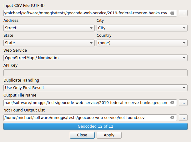
- Input CSV File: Table of addresses to geocode. This file should be encoded in the UTF-8 character set. Although other 8-bit encodings (like Windoze ISO-8859-x) will work if only ASCII characters are present, non-ASCII characters may cause unpredictable behavior.
- Address, City, State, and Country: Selected columns from the input CSV file are added as attributes in the output shapefile. Addresses may be spread across as many as four different columns. However, these fields are concatenated into a single address to query the API, so only one meaningful column is absolutely required (such as for a city/state combination).
- Web Service: See the associated pages for volume limits and terms of service:
- API Key: To use the paid services, you will need an API key:
- ESRI Server URL: When using an ESRI Server for geocoding, a server URL must
be provided. Publicly accessible servers include:
- ArcGIS World Geocoding Service: https://geocode.arcgis.com/arcgis/rest/services/World/GeocodeServer/findAddressCandidates
- NY State GIS Program Office Geocoding Service: https://gisservices.its.ny.gov/arcgis/rest/services/Locators/Street_and_Address_Composite/GeocodeServer/findAddressCandidates
- Duplicate Handling: This parameter indicates how to handle conditions where
- Use Only First Result
- Multiple Features For Multiple Results: Note that geocoders often return multiple locations representing different spatial scales (street address, city centroid, state centroid, etc.). Therefore, use of this option will likely require extensive editing of the results to cull unneeded points
- Output File Name: The name of the output feature file
- Not Found Output List: A CSV file that will contain input lines that could not be geocoded
Python
mmqgis_geocode_web_service(input_csv_name, parameter_attributes, web_service,
	api_key, use_first, output_file_name, not_found_file_name, status_callback = None)
parameter_attributes is a list of tuples mapping fields in the CSV file to one of the following address fields: Address, City, State, Country.
The following example geocodes the 12 US Federal Reserve Banks using Nominatim.
- Bank table: 2019-federal-reserve-banks.csv
input_csv_name = "2019-federal-reserve-banks.csv"
parameter_attributes = [ ("Address", "Street"), ("City", "City"), ("State", "State") ]
web_service = "OpenStreetMap / Nominatim"
api_key = None
use_first = True
output_file_name = "2019-federal-reserve-banks.geojson"
not_found_file_name = "2019-federal-reserve-banks.notfound.csv"

message = mmqgis_geocode_web_service(input_csv_name, \
	parameter_attributes, web_service, api_key, use_first, \
	output_file_name, not_found_file_name)

print("Geocode: " + str(message))
The following example geocodes the same locations using the Google geocoder.
input_csv_name = "2019-federal-reserve-banks.csv"
parameter_attributes = [ ("Address", "Street"), ("City", "City"), ("State", "State") ]
web_service = "Google"
api_key = "YOUR API KEY HERE"
use_first = True
output_file_name = "2019-federal-reserve-banks.geojson"
not_found_file_name = "2019-federal-reserve-banks.notfound.csv"

message = mmqgis_geocode_web_service(input_csv_name, \
	parameter_attributes, web_service, api_key, use_first, \
	output_file_name, not_found_file_name)

print("Geocode: " + str(message))
The following example geocodes the same locations using the ArGIS World Geocoding Service.
input_csv_name = "2019-federal-reserve-banks.csv"
parameter_attributes = [ ("Address", "Street"), ("City", "City"), ("State", "State") ]
web_service = "ESRI Server"
api_key = "https://geocode.arcgis.com/arcgis/rest/services/World/GeocodeServer/findAddressCandidates"
use_first = True
output_file_name = "2019-federal-reserve-banks.geojson"
not_found_file_name = "2019-federal-reserve-banks.notfound.csv"

message = mmqgis_geocode_web_service(input_csv_name, \
	parameter_attributes, web_service, api_key, use_first, \
	output_file_name, not_found_file_name)

print("Geocode: " + str(message))
Geocode from Street Layer
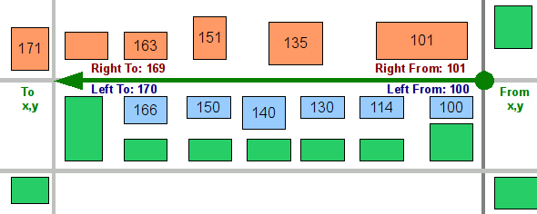
The Geocode Street Layer tool geocodes addresses from a CSV file using an address locator layer with street centerline features and attributes indicating the range of addresses associated with each feature.
Examples of street centerline files include:
- The US Census Bureau TIGER/Line All Lines shapefiles
- New York City Department of City Planning LION files
- Geodatabases created as ESRI address locators
As with many tools of this type, the matching and interpolation is quite fragile. Street names in the street layer generally must match the names in the CSV file exactly - First Street may not match 1st Street.
The tool will also only handle address street numbers that are entirely numeric. Hyphenated (172-10 Seventh Ave) or fractional nubers (1872a Main) will generally not match, although line files for areas with hyphenated numbers will often have a field with the hyphens removed.
To improve matching, street names are internally modified with common abbreviations such as st for street and w for west. This add fuzziness to the search process that improves the hit ratio but may result in unexpected results. This address handling may be augmented or refined in future releases.
Parameters
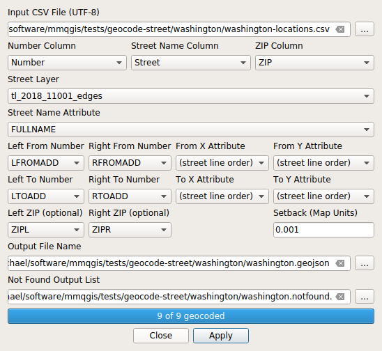
- Input CSV File: The input address CSV file. This file should be encoded in the UTF-8 character set. Although other 8-bit encodings (like Windoze ISO-8859-x) will work if only ASCII characters are present, non-ASCII characters may cause unpredictable behavior
- Number Column: The file of addresses should separate the numeric street address numbers from the street names. The name of the column in the CSV file containing the street address numbers
- Street Name Column: The name of the column in the CSV file containing the street names. While the tool will attempt to normalize street names so they are comparable, the matching process is usually fuzzy and imperfect
- ZIP Column (optional): The name of the column in the CSV file containing ZIP Codes
- Street Layer: The map layer containing the street centerline features
- Street Name Attribute: The name of the field in the street layer containing street names
- Left From Number / Left To Number: The names of the fields in the street layers indicating the range of street address numbers on the left side of the street. Left and right are determined by the order of nodes that make up each linestring. If one side of the street has odd numbers and the other has even, the to/from numbers should also be odd or even
- Left ZIP (optional): The name of the field in the street layer indicating the ZIP Code on the left side of the street
- Right From Number / Right To Number: The names of the fields in the street layers indicating the range of street address numbers on the rightside of the street. Left and right are determined by the order of nodes that make up each linestring. If one side of the street has odd numbers and the other has even, the to/from numbers should also be odd or even
- Right ZIP (optional): The name of the field in the street layer indicating the ZIP Code on the right side of the street
- From X Attribute, From Y Attribute, To X Attribute, To Y Attribute (optional): Each street layer feature can also have an associated line indicating the locations of buildings relative to the street so that geocoded points are placed closer to the building locations rather than in the middle of streets
- Setback (optional): If given, points will be offset from street centerlines and intersections by this distance in map units. If the street layer is in WGS 84 latitude/longitude, setback distances can only be approximated, and this value should usually be quite small, such as 0.0001 or 0.0002.
- Output File Name: The name of the output file where geocoded features will be saved. In addition to all columns from the input CSV file, fields for Latitude, Longitude, and Side (left or right) will be added for diagnostics
- Not Found Output List: The name of a CSV file for addresses that cannot be found in the street layer
Python
mmqgis_geocode_street_layer(input_csv_name, number_column, street_name_column, zip_column, \
	input_layer, street_name_attr, left_from_attr, left_to_attr, left_zip_attr, \
	right_from_attr, right_to_attr, right_zip_attr, \
	from_x_attr, from_y_attr, to_x_attr, to_y_attr, setback, \
	output_file_name, not_found_file, status_callback = None)
The following example geocodes a file of addresses in Washington, DC using a US Census Bureau TIGER/Line All Lines shapefile.
input_csv_name = "washington-locations.csv"
number_column = "Number"
street_name_column = "Street"
zip_column = "ZIP"

input_layer_name = "tl_2018_11001_edges.shp"
input_layer = QgsVectorLayer(input_layer_name)
street_name_attr = "FULLNAME"
left_from_attr = "LFROMADD"
left_to_attr = "LTOADD"
left_zip_attr = "ZIPL"
right_from_attr = "RFROMADD"
right_to_attr = "RTOADD"
right_zip_attr = "ZIPR"

from_x_attr = None
from_y_attr = None
to_x_attr = None
to_y_attr = None
setback = 0.0001

output_file_name = "washington.geojson"
not_found_file = "washington-not-found.csv"

message = mmqgis_geocode_street_layer(input_csv_name, \
	number_column, street_name_column, zip_column, \
	input_layer, street_name_attr, left_from_attr, left_to_attr, left_zip_attr, \
	right_from_attr, right_to_attr, right_zip_attr, \
	from_x_attr, from_y_attr, to_x_attr, to_y_attr, setback, \
	output_file_name, not_found_file)

print("Geocode Street Layer: " + str(message))
Reverse Geocode
The Reverse Geocode tool uses Google or Nominatim (OpenStreetMap) API to find addresses associated with point feature locations. If features are lines or polygons, the centroid of each feature will be used for querying.
Additional attributes are added to each feature to preserve what the web service geocoded so that accuracy can be assessed. These attributes are dependent upon the geocoder used:
- Google
- result_num: The index of the result when multiple results are returned for a single address
- status: Always OK
- formatted_address: The address as found by the API
- place_id: Internal Google identifier
- location_type: Additional data about the location, such as ROOFTOP or APPROXIMATE
- latlong: The latitude, longitude found by the API
- OpenStreetMap / Nominatim:
- result_num: The index of the result when multiple results are returned for a single address
- osm_id: OpenStreetMap ID number
- display_name: The OSM address for the location
- category: The category of feature found
- type: The type within the category given above
- latlong: The latitude, longitude found by the API
Parameters
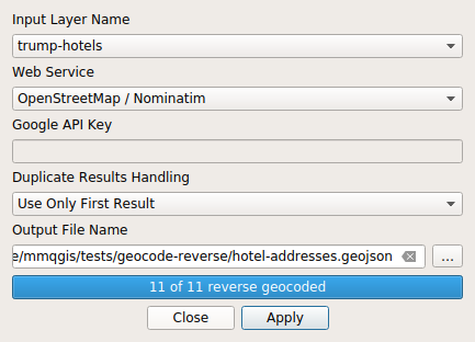
- Input Layer Name: The map layer containing the features that you wish to find street addresses for
- Web Service: Google or OpenStreetMap / Nominatim
- API Key: To use the Google geocoder, you will need to get an API key and include it in the API Key field
- Duplicate Results Handling: Use Only First Result or Multiple Features for Multiple Results. Note that the latter can include locations for enclosing areas like streets, cities, states, etc. which may make your search results too cluttered to be useful
- Output File Name: A file that will contain point features and attributes from the input layer, along with an address field containing the reverse geocoded addresses
Python
mmqgis_geocode_reverse(input_layer, web_service, api_key, use_first,
	output_file_name, status_callback = None)
The following example finds addresses for an input layer of hotel points.
input_file_name = "trump-hotels.geojson"
input_layer = QgsVectorLayer(input_file_name)
web_service = "OpenStreetMap / Nominatim"
api_key = None
use_first = False
output_file_name = "hotel-addresses.geojson"

message = mmqgis_geocode_reverse(input_layer, web_service, api_key, use_first, \
		output_file_name, output_file_format)

print("Reverse geocode OSM: " + str(message))
Import / Export Tools
Attributes Export to CSV File
The Export Attributes tool saves attributes from a map layer to a CSV file, which can then be viewed or edited. This can be helpful when you have some use for the attribute data without the associated geographic data.
This tool is largely duplicates the QGIS native export function (right click on a layer and choose Export). This tool is a legacy of prior QGIS versions that did not have robust export capabilities, and this tool is preserved for folks who like a somewhat simpler user interface.
Parameters
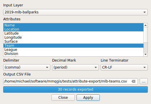
- Input Layer: Name of the map layer containing attributes to export
- Attributes: A multiple-selection list box on the dialog permits selection of the attribute columns to export. Hold the CTRL key down to select multiple fields
- Delimiter: Output file field delimiter - comma, semicolon, or space
- Decimal Mark: Output file decimal mark - period (US) or comma (Europe)
- Line Terminator: Output file line terminator character(s) - CR-LF (Windows) or LF (Mac / Linux)
- Output CSV File: Output file name
Python
mmqgis_attribute_export(input_layer, attribute_names, output_csv_name, \
			field_delimiter = ",", line_terminator = "\n", decimal_mark = ".", \
			status_callback = None)
The example below exports team name attributes from a list of MLB ballparks.
- MLB ballpark locations from Wikipedia: 2019-mlb-ballparks.geojson
input_layer_name = "2019-mlb-ballparks.geojson"
input_layer = QgsVectorLayer(input_layer_name)
attribute_names = ["Team", "Location", "Name"]
output_csv_name = "mlb-teams.csv"
field_delimiter = ";"
line_terminator = "\n"
decimal_mark = "."

message = mmqgis_attribute_export(input_layer, attribute_names, output_csv_name, \
		field_delimiter, line_terminator, decimal_mark, status_callback)

print("Export Attributes: " + str(message))
Geometry Export To CSV
The Geometry Export To CSV tool exports points, polylines or polygons to comma-separated variable (CSV) files. Two separate files are created: a node file and an attribute file. This tool is useful for inspecting geometries.
The output node file contains the following columns:
- shapeid: A sequential number of features in the file
- partid: The number of the part in multi-part geometries. This will always be zero with single-part geometries
- x: The longitude or northing
- y: The latitude or easting
The output attribute file contains all attributes from the source features, plus a shapeid column that associates those attributes with nodes in the node file.
For simple point features, the attributes are included in the node file and no attribute file is created.
Geometries exported using this tool can be re-imported using the Geometry Import from CSV tool.
Note that the two-file CSV format used by this tool is different from the single-file GeoCSV format that stores geometries in a column of Well-Known Text (WKT). GeoCSV files can be created with the native QGIS export function.
Parameters
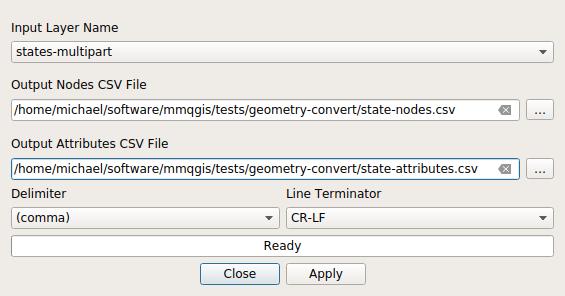
- Input Layer Name: The name of the map layer to export
- Output Nodes CSV File: The name of the node file
- Output Attributes CSV File: The name of the attribute file
- Delimiter: The CSV field delimiter - comma, semicolon, or space
- Line Terminator: Output file line terminator character(s) - CR-LF (Windows) or LF (Mac / Linux)
Python
mmqgis_geometry_export_to_csv(input_layer, node_file_name, attribute_file_name, \
		field_delimiter = ",", line_terminator = "\n", status_callback = None)
The following example exports a shapefile of US states to CSV geometry files.
layer_file_name = "states-multipart.shp"
input_layer = QgsVectorLayer(layer_file_name)
node_file_name = "states-nodes.csv"
attribute_file_name = "states-attributes.csv"
field_delimiter = ","
line_terminator = "\n"
message = mmqgis_geometry_export_to_csv(input_layer, node_file_name, \
	attribute_file_name, field_delimiter, line_terminator)

print("Export Geometry to CSV: " + str(message))
Geometry Import From CSV
The Geometry Import From CSV tool imports points, polylines, and polygons from comma-separated variable (CSV) files of X/Y nodes.
Other than providing a compliment to the Geometry Export To CSV tool described above, this command can be used to import transit "shapes.txt" data from General Transit Feed Specification (GTFS) releases by transit agencies.
The input CSV file(s) should be encoded in the UTF-8 character set. Although other 8-bit encodings (like Windoze ISO-8859-x) will work if only ASCII characters are present, non-ASCII characters may cause unpredictable behavior.
For point layers, only a single input CSV file is needed that includes latitude and longitude columns. All other columns are imported as attributes. This is essentially the same as the Add Delimited Text Layer native QGIS command. Files are read using the QgsVectorLayer() constructor. Attributes imported as text strings may be converted to floating point using the MMQGIS Text to Float tool.
For polyline and polygon layers, individual nodes of each shape should be provided on separate rows in an input CSV node file. The file should have three columns: Latitude, Longitude, and Shape ID. Any additional columns will be ignored. Nodes for each shape should have the same unique Shape ID value and should occur in the file in the same sequence that they will be added to the shape.
If the imported polylines or polygons have additional attributes to be imported, they should be placed in a separate CSV file with a Shape ID column to join to the imported nodes using the MMQGIS Attributes Join From CSV File command.
Parameters
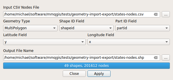
- Input CSV Nodes File: A CSV file of x/y nodes that will be imported as features
- Geometry Type: The type of geometry to create from the nodes
- Point
- LineString
- Polygon
- MultiPoint
- MultiLineString
- MultiPolygon
- Shape ID Field: The name of the field in the CSV file containing the shape IDs. Shape IDs are used for grouping nodes by feature
- Part ID Field: The name of the field in the CSV file containing the part IDs. Part IDs are used for grouping nodes by part within each feature. Not needed for single part geometries.
- Latitude Field: The name of the field in the CSV file containing latitudes / northings
- Longitude Field: The name of the field in the CSV file containing longitudes / eastings
- Output File Name: The name of the file where the imported features will be saved
Python
mmqgis_geometry_import_from_csv(input_csv_name, shape_id_field, part_id_field, \
		geometry_type, latitude_field, longitude_field, \
		output_file_name, status_callback = None)
The following example imports a CSV file of state boundary nodes as multipolygons and then joins attributes to recreate the layer. This is the compliment of the Geometry Export To CSV File example given above.
shape_id_field = "shapeid"
part_id_field = "partid"
geometry_type = "MultiPolygon"
latitude_field = "y"
longitude_field = "x"
output_file_name = "states-nodes.geojson"

message = mmqgis_geometry_import_from_csv(node_file_name, \
		shape_id_field, part_id_field, \
		geometry_type, latitude_field, longitude_field, \
		output_file_name)

print("Import Geometries: " + str(message))

input_layer_name = "states-nodes.geojson"
input_layer = QgsVectorLayer(input_layer_name)
input_layer_attribute = "shapeid"
input_csv_name = "states-attributes.csv"
input_csv_attribute = "shapeid"
output_file_name = "new-states.geojson"

message = mmqgis_attribute_join(input_layer, input_layer_attribute, \
		input_csv_name, input_csv_attribute, output_file_name)

print("Attribute Join: " + str(message))
KML Export
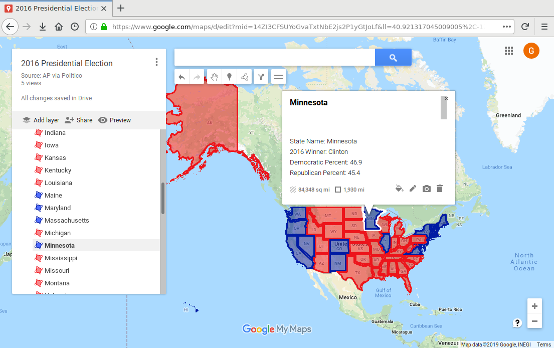
The KML Export tool exports features to KML with the capability to explicitly specify fields for the name and description that are always displayed in the Google Maps interface. This tool also styles the KML in an approximation of the symbology configured for the exported layer
Although you can import and export KML in QGIS natively, the OGR/GDAL library used by QGIS does not give strong control over symbology, the name field, or the description field that are displayed in Google Maps.
This tool exports points using the default Google Maps PNG icons. Since a full palette of icon colors is not available, icon colors are approximated based on the RGB values of point layer symbol colors.
Note that Google Maps has a KML size limit of 5 MB. If your layer has highly-detailed polygons, you may need to simplify your geometries using the MMQGIS Gridify tool or the Processing vector geometry Simplify tool.
Parameters
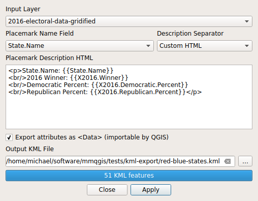
- Input Layer: The name of the layer to export as KML
- Placemark Name Field: The layer field name used as the Name of placemarks
- Description Separator: The format in which fields are included in the placemark Description:
- Field Names: All field names and values are placed in a single HTML paragraph with line breaks before each field
- Paragraphs: All field names and values are placed in separate paragraphs for each field
- Commas: All field values (no names) are placed in a single paragraph with values separated with commas
- Custom HTML: The description contains HTML you define, with field values enclosed in double braces
<p>State Name: {{State.Name}}
<br/>2016 Winner: {{X2016.Winner}}
<br/>Democratic Percent: {{X2016.Democratic.Percent}}
<br/>Republican Percent: {{X2016.Republican.Percent}}</p>
Python
mmqgis_kml_export(input_layer, name_field, description, export_data,
		  output_file_name, status_callback = None)
The example below creates a red vs blue state KML file using styling defined in the script.
- Election Data: 2016-electoral-data.geojson
# Gridify (simplify) to keep final file under the Google Maps 5 MB limit
input_layer_name = "2016-electoral-data.geojson"
input_layer = QgsVectorLayer(input_layer_name)
horizontal_spacing = 0.01
vertical_spacing = 0.01
temp_file_name = "temp-states.geojson"

message = mmqgis_gridify_layer(input_layer, horizontal_spacing, \
			vertical_spacing, temp_file_name)
print("Gridify: " + str(message))


# Define the styling for the renderer
red_fill = QgsFillSymbol.createSimple({'color': '#800000', 'outline_color': 'black'})
blue_fill = QgsFillSymbol.createSimple({'color': '#000080', 'outline_color': 'black'})

choropleth_renderer = QgsCategorizedSymbolRenderer("X2016.Winner")
choropleth_renderer.addCategory(QgsRendererCategory("Trump", red_fill, "Trump"))
choropleth_renderer.addCategory(QgsRendererCategory("Clinton", blue_fill, "Clinton"))

# Load the gridified file
input_layer = QgsVectorLayer(temp_file_name)
input_layer.setRenderer(choropleth_renderer)
input_layer.setOpacity(0.5)

# Export to KML
name_field = "State.Name"
description = "<p>State Name: {{State.Name}}" + \
	"<br/>2016 Winner: {{X2016.Winner}}" + \
	"<br/>Democratic Percent: {{X2016.Democratic.Percent}}" + \
	"<br/>Republican Percent: {{X2016.Republican.Percent}}</p>"
export_data = False
output_file_name = "red-blue-states.kml"

message = mmqgis_kml_export(input_layer, name_field, description, export_data, output_file_name, status_callback)
print("KML Export: " + str(message))
The code can be simplified if you get your styling from a QGIS project file.
# This must be a full path name (not relative) or the layers will not load
project_file = "/home/michael/software/mmqgis/tests/kml-export/kml-export.qgs"
project = QgsProject.instance()
project.read(project_file)
input_layer = project.mapLayersByName("2016-electoral-data-gridified")[0]

name_field = "State.Name"
description = "<p>State Name: {{State.Name}}" + \
	"<br/>2016 Winner: {{X2016.Winner}}" + \
	"<br/>Democratic Percent: {{X2016.Democratic.Percent}}" + \
	"<br/>Republican Percent: {{X2016.Republican.Percent}}</p>"
export_data = False
output_file_name = "red-blue-states2.kml"

message = mmqgis_kml_export(input_layer, name_field, description, \
		export_data, output_file_name)

print("KML Export From a Project File: " + str(message))
Modify Tools
Change Projection
The Change Projection tool changes the projection (reprojects) a layer to a new projection and transforms the geometries of all features in that layer to the new projection.
The dialog displays the PROJ string for the existing and new projections.
This tool largely duplicates the capabilities of the Reproject layer tool from the Processing toolkit.
Parameters
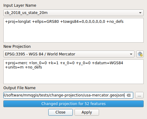
- Input Layer Name: The name of the map layer that will have its projection changed
- New Projection: The name of the new projection. Click the drop-down to select from previously used projections or click the globe icon to select from the list of all available projections
- Output File Name: The name of the output file for the reprojected features
Python
mmqgis_change_projection(input_layer, new_crs, output_file_name, status_callback = None)
The example below changes the projection of a USCB cartographic boundary file for the US to a North American Albers projection:
input_layer_name = "cb_2018_us_state_20m.shp"
input_layer = QgsVectorLayer(input_layer_name)

new_crs = QgsCoordinateReferenceSystem("PROJ4:+proj=aea +lat_1=20 +lat_2=60 " + \
	"+lat_0=40 +lon_0=-96 +x_0=0 +y_0=0 +datum=NAD83 +units=m +no_defs")
output_file_name = "usa-albers.geojson"

message = mmqgis_change_projection(input_layer, new_crs, output_file_name)
print("Change projection: " + str(message))
Convert Geometry
The Geometry Convert tool changes the geometry types of shapes.
- All shapes other than points can be converted to centroids or individual node points
- Multi-part shapes (multi-point, multi-line, multi-polygon) can be decomposed to individual parts (point, line, polygon, respectively)
- Single-part shapes can be merged into multi-part shapes based on a common attribute (Merge Field). Numeric attributes from from the multiple source features will be handled using the Merge Attribute Operation (First or Sum). String attributes from multiple source features are always merged using the value from the first encountered feature.
- Polygons and multi-polygons can be converted to lines
- Shapes with elevation (2.5-D) are converted to X/Y (2-D). This can be helpful for converting GPS or KML layers to 2-D for merging with other 2-D layers (elevation is discarded)
Parameters
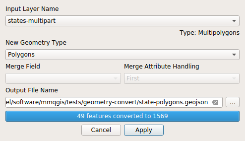
- Input Layer Name: The name of the layer containing geometries to convert
- New Geometry Type: The type of geometry that the layer will be converted to
- Merge Field: The name of the field in the input layer used to specify which single parts should be merged into multipart geometries. Only needed when converting from singlepart to multipart
- Merge Attribute Handing: How to combine attributes when merging parts - First or Sum
- Output File Name: The name of the file where the features with new geometries will be saved
Python
mmqgis_geometry_convert(input_layer, new_geometry, output_file_name, status_callback = None)
The following breaks a multipart state file (including islands) into single parts.
input_layer_name = "states-multipart.shp"
input_layer = QgsVectorLayer(input_layer_name)
new_geometry = "Polygons"
output_file_name = "state-polygons.geojson"
message = mmqgis_geometry_convert(input_layer, new_geometry, output_file_name)
print("Multipolygons to Polygons: " + str(message))
Delete Duplicate Geometries
The Delete Duplicate Geometries tool removes duplicate features from a layer. Two features are considered duplicates if their geometries are exactly identical, as determined by the QgsGeometry equals() function. Attributes are not considered, only geometry.
To improve speed, this tool loads all geometries into memory - which may cause memory issues with large datasets or large numbers of complex polygons.
Parameters
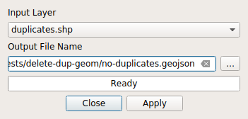
- Input Layer: The name of the map layer from which you want to remove duplicate features
- Output File Name: The name of the file where the non-duplicated features will be saved
Python
mmqgis_delete_duplicate_geometries(input_layer, output_file_name, status_callback = None)
This example removes duplicates from a layer.
	layer_file = "duplicates.shp"
	input_layer = QgsVectorLayer(layer_file)
	output_file_name = "no-duplicates.geojson"

	message = mmqgis_delete_duplicate_geometries(input_layer, output_file_name)

	print("Delete duplicate geometries: " + str(message))
Float to Text
The Float to Text tool converts integer and floating point values to strings, with the ability to specify thousands separators, the number of decimal digits, prefixes and suffixes (eg. dollar sign prefix or "miles" suffix). This is the opposite of the Text to Float tool.
Parameters
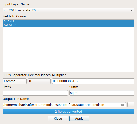
- Input Layer Name: The name of the map layer containing fields to convert to text
- Fields to Convert: The name of the fields to convert
- 000's Separator: Comma (US) or Space (EU)
- Decimal Places: The number of decimal places
- Multiplier: A value to multiply the numeric values by. Useful for unit conversion or scaling
- Prefix: Optional text to place before the number (such as monetary units)
- Suffix: Optional text to place after the number (such as distance units)
- Output File Name: Name of the file to write the data with converted fields
Python
 mmqgis_float_to_text(input_layer, attributes, separator, \
			 decimals, prefix, suffix, multiplier, \
		 	 output_file_name, status_callback = None)
The following converts land and water areas from square meters to square miles from a US Census Bureau state cartographic boundary file.
input_layer_name = "cb_2018_us_state_20m.shp"
input_layer = QgsVectorLayer(layer_file)
attributes = ["ALAND", "AWATER"]
separator = ","
decimals = 2
multiplier = 0.000000386102
prefix = None
suffix = " sq mi"
output_file_name = "state-area.geojson"

message = mmqgis_float_to_text(input_layer, attributes, separator, \
	decimals, prefix, suffix, output_file_name)

print("Float to Text: " + str(message))
Gridify
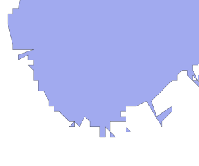
The Gridify tool simplifies points, lines and polygons in a shapefile by aligning all vertices to a specified grid and then removing redundant points.
Gridification makes it possible to significantly improve display refresh time when working with shapefiles that are more detailed than is necessary for the final map. However, the gridification process can result in some odd artifacts when viewed at higher resolutions, particularly in dealing with coves and other appendages along the edges of larger polygons.
Parameters
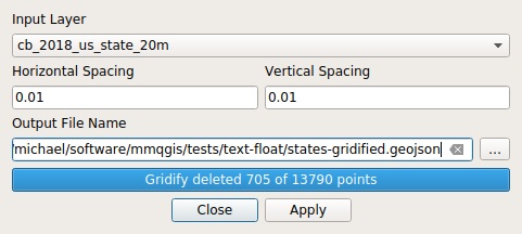
- Input Layer: The name of the map layer to gridify
- Horizontal Spacing / Vertical Spacing: Specification of the alignment grid. Defaults are based on 0.5% of the extent of the target layer
- Output File Name: Output file for the gridified shapes
Python
mmqgis_gridify_layer(input_layer, horizontal_spacing, vertical_spacing,
		     output_file_name, status_callback = None)
The following example gridifies a file of US states to reduce the size so it can be exported to KML.
# Gridify (simplify) to keep final file under the Google Maps 5 MB limit
input_layer_name = "2016-electoral-data.geojson"
input_layer = QgsVectorLayer(input_layer_name)
horizontal_spacing = 0.01
vertical_spacing = 0.01
temp_file_name = "temp-states.geojson"

message = mmqgis_gridify_layer(input_layer, horizontal_spacing, \
			vertical_spacing, temp_file_name)
print("Gridify: " + str(message))
Sort
The Sort tool sorts features in the data. Although the QGIS Open Attribute Table feature can sort displayed attributes dynamically by any field, the Sort tool can make exported attributes easier to browse and analyze.
Parameters
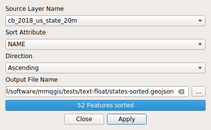
- Source Layer Name: The layer to sort
- Sort Attribute: The field to sort by
- Direction: Sort direction - Ascending or Descending
- Output File Name: The output file where the sorted data will be saved
Python
mmqgis_sort(input_layer, sort_field, sort_direction, output_file_name, status_callback = None)
The following example sorts a file of states by name.
input_layer_name = "statesp020.shp"
input_layer = QgsVectorLayer(input_layer_name)
sort_field = "STATE"
sort_direction = "Ascending"
output_file_name = "states-sorted.geojson"

message = mmqgis_sort(input_layer, sort_field, sort_direction, output_file_name)

print("Ascending sort: " + str(message))
Text to Float
The Text to Float tool converts string attributes to floating point. This tool is useful for imported data where numeric fields are stored as strings and contain extraneous non-numeric characters like currency symbols, thousands separators, and/or footnote marks.
Parameters
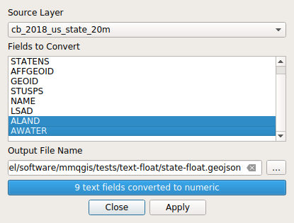
- Source Layer: The layer containing the fields for conversion
- Fields to Convert: Select the attributes to be converted. Multiple fields may be selected
using the shift and control keys. Care should be exercised in selecting fields since fields containing
strings that cannot be converted to floating point (e.g. strings with
non-numeric characters) will be assumed to have a value of zero.
Integer fields are converted to floating point, which should result in no loss of precision but may increase shapefile size. However, integer strings exceeding MAXINT will get unpredictable values and there may be some loss of precision when converting real values with large numbers of digits of significance.
- Output File Name: The name of the file where the modified data will be saved
Python
mmqgis_text_to_float(input_layer, field_names, output_file_name, status_callback = None)
The following example converts the land and water area fields back to numeric fields. This is the opposite of the Float to Text example above.
input_layer_name = "state-area.geojson"
input_layer = QgsVectorLayer(layer_file)
field_names = ["ALAND", "AWATER"]
output_file_name = "state-float.geojson"

message = mmqgis_text_to_float(input_layer, field_names, output_file_name)

print("Text to Float: " + str(message))
Search / Select
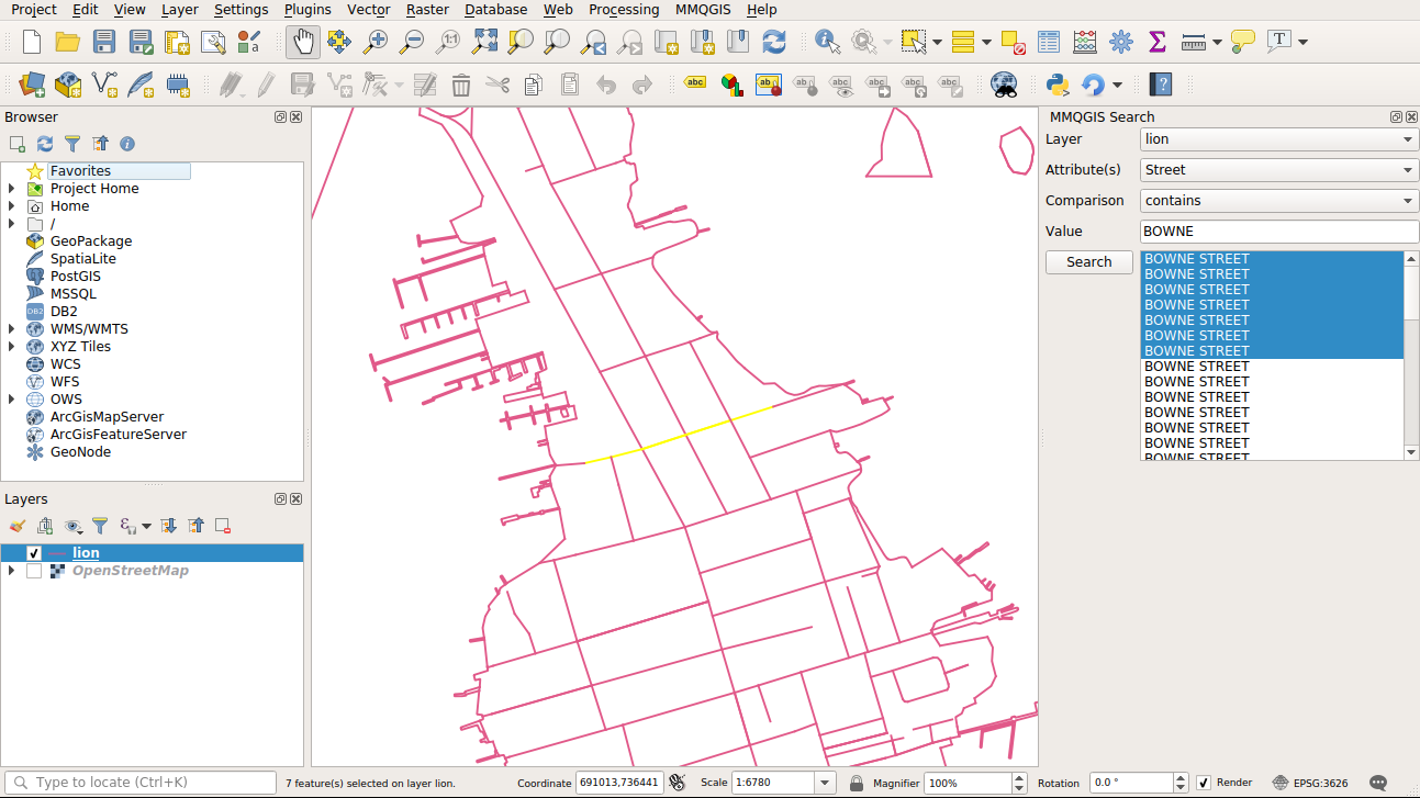
The Search / Select widget permits interactive browsing of features that match the specified search criteria. Results are displayed in a list box in the search widget.
Clicking one of the features on the results box moves the map canvas to center that feature in the window.
This tool also provides options in the layer selection combo box for searching addresses using Nominatim / Open Street Map. Selection of an address only pans the map display to place the location in the center of the display, and no markings are added to the map.
Multiple selections in the results list are possible using the CTRL and SHIFT keys. If multiple features are selected, the map canvas centers on a central area between the centroids of all selected features.
Layer feature searches can be made on one specific attribute field in one specific layer, across all layers by choosing [All Layers] in the layers combo box, and/or all fields in the specified layers by choosing the [all] attributes option in the attribute combo box. Choosing to search all layers or attributes can be time-consuming, and/or yield an unmanageable set of search result features.
Possible comparisons on numeric or string attributes are the common permutations of equal, greater than, or less than. String attributes can be searched with "contains" or "begins with." Searches are case insensitive.
Python
The search widget is an interactive tool that is integrated with the QGIS user interface and does not have a library function. You can perform searches on layers with expressions using methods like QgsVectorLayer.getFeatures().
Programming with MMQGIS
Console Programming
MMQGIS tools are built around Python functions that can be used from the QGIS Python console by importing the mmqgis_library.py functions from the plugin directory using the import command. Output feature files can then be added to the current map project using the iface.addVectorLayer() function.
The following example uses the mmqgis_grid() code snippet from above to create and add a 10-degree graticule layer to the current project:
from mmqgis.mmqgis_library import *

geometry_type = "Lines"
crs = QgsCoordinateReferenceSystem("PROJ4:+proj=longlat +datum=WGS84 +no_defs")
x_spacing = 10
y_spacing = 10
x_left = -170
x_right = 170
y_bottom = -80
y_top = 80
output_file_name = "world-grid.geojson"

mmqgis_grid(geometry_type, crs, x_spacing, y_spacing, x_left, y_bottom, x_right, y_top, output_file_name)

iface.addVectorLayer(output_file_name, "Graticule", "ogr")
QGIS Python Console Scripts
Your code can also be placed in external script files and executed from the QGIS Python console.
For example, if you create a script such as the one above and place it in a file, you can execute it in the QGIS python console in the same way you would execute scripts from the Python interpreter shell:
exec(open("/home/michael/test.py").read())
Note that you should only use exit() commands in your script if you want to exit QGIS as well.
Stand-Alone Programming
QGIS library functions and MMQGIS tools can also be used in stand-alone Python scripts that you can run without having to start QGIS. You need to include the following code at the beginning of your script to load the QGIS libraries and create a QGIS instance:
from qgis.core import *
qgs = QgsApplication([], True)
qgs.initQgis()
As with console scripts, you need to import the mmqgis_library module. However, you may need to add the directory containing mmqgis_library.py to your sys.path.
The example below is a version of the grid script given above that can be executed from a stand-alone Python script. The folder added to sys.path will differ depending on where MMQGIS is installed on your system.
from qgis.core import *
qgis = QgsApplication([], True)
qgis.initQgis()

import sys
sys.path.append("/home/michael/software/mmqgis/")
from mmqgis_library import *

geometry_type = "Lines"
crs = QgsCoordinateReferenceSystem("PROJ4:+proj=longlat +datum=WGS84 +no_defs")
x_spacing = 10
y_spacing = 10
x_left = -170
x_right = 170
y_bottom = -80
y_top = 80
output_file_name = "world-grid.geojson"

mmqgis_grid(geometry_type, crs, x_spacing, y_spacing, x_left, y_bottom, x_right, y_top, output_file_name)
Multiple File Operations
One of the major strengths of scripting is the ability to perform the same operation on multiple data files.
You can explicitly specify multiple files in an array. For example, this script changes the projection on a set of files to WGS 84 latitude/longitude.
from qgis.core import *
qgis = QgsApplication([], True)
qgis.initQgis()

from mmqgis_library import *

input_file_names = [ "alpha.shp", "beta.shp", "gamma.shp" ]

wgs84 = QgsCoordinateReferenceSystem("PROJ4:+proj=longlat +datum=WGS84 +no_defs")

for input_file_name in input_file_names:
	input_layer = QgsVectorLayer(input_file_name)
	output_file_name = input_file_name.replace(".shp", "-reprojected.shp")
	message = mmqgis_change_projection(input_layer, wgs84, output_file_name)
	print(input_file_name + " = " + output_file_name + " = " + str(message))
You can also use the Python scandir() function to get a list of files in a directory.
from qgis.core import *
qgis = QgsApplication([], True)
qgis.initQgis()

from mmqgis_library import *

import os
os.chdir("tests/batch")

input_file_names = []
for input_file_name in os.scandir("."):
	if input_file_name.name[-4:] == ".shp":
		input_file_names.append(input_file_name.name)

wgs84 = QgsCoordinateReferenceSystem("PROJ4:+proj=longlat +datum=WGS84 +no_defs")

for input_file_name in input_file_names:
	input_layer = QgsVectorLayer(input_file_name)
	output_file_name = input_file_name.replace(".shp", "-reprojected.shp")
	message = mmqgis_change_projection(input_layer, wgs84, output_file_name)
	print(input_file_name + " = " + output_file_name + " = " + str(message))
Status Callback
All MMQGIS library functions have an optional status_callback parameter that permits display of status messages as the tool completes and provides a way of terminating tools when they exceed a time limit. The callback function had two parameters: the percent completed and a string status message.
This example defines a simple status_callback that prints status messages to the screen.
from qgis.core import *
qgis = QgsApplication([], True)
qgis.initQgis()

from mmqgis_library import *

import os
os.chdir("tests/batch")

def status_callback(percent, message):
	print("\t" + str(int(percent)) + "%: " + message)
	return 0

input_file_names = []
for input_file_name in os.scandir("."):
	if os.path.splitext(input_file_name.name)[1] == ".shp":
		input_file_names.append(input_file_name.name)

wgs84 = QgsCoordinateReferenceSystem("PROJ4:+proj=longlat +datum=WGS84 +no_defs")

for input_file_name in input_file_names:
	input_layer = QgsVectorLayer(input_file_name)
	output_file_name = input_file_name.replace(".shp", "-reprojected.shp")
	message = mmqgis_change_projection(input_layer, wgs84, output_file_name)
	print(input_file_name + " = " + output_file_name + " = " + str(message))
Image File Output
Layers can be exported as maps to PNG files. The easiest course of action is to set up the print layout in the layout editor in QGIS and then use that layout from the project file in your script.
These examples use election data from the AP via Politico: 2016-electoral-data.geojson
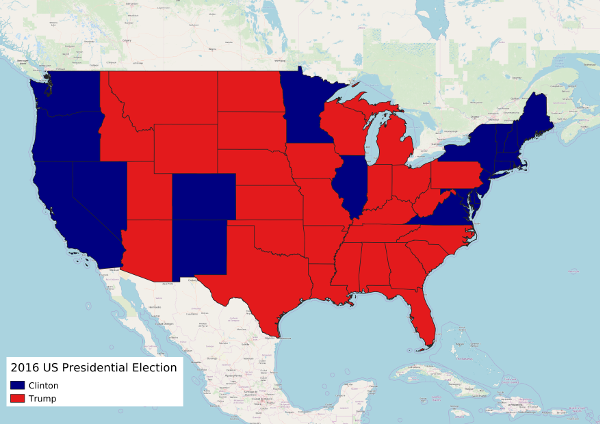
from qgis.core import *
qgis = QgsApplication([], True)
qgis.initQgis()

# Load the project
# This needs to be a full path, otherwise layers do not get read in
project_file = "/home/michael/software/mmqgis/tests/kml-export/2016-election-osm-map.qgs"
project = QgsProject.instance()
project.read(project_file)
if project.error():
	exit("Error: " + project.error())

# Get the print layout from the project
print_layout = QgsProject.instance().layoutManager().printLayouts()[0]

# Create an exporter and export the layout to a PNG file
exporter = QgsLayoutExporter(print_layout)
exporter.exportToImage("2016-election-osm-map.png", exporter.ImageExportSettings())
However, if you are batch exporting images from a variety of different layers, you need programmatic control of your layout, or you just want to setup a print layout that you can duplicate and modify without having to use the QGIS interface, you can define print layouts in Python, although these are cumbersome for complex symbology and/or layouts.
# Create the OpenStreetMap tiled base map
osm_url = 'type=xyz&url=https://a.tile.openstreetmap.org/' +\
	'%7Bz%7D/%7Bx%7D/%7By%7D.png&zmax=19&zmin=0&crs=EPSG3857'
osm_layer = QgsRasterLayer(osm_url, 'OpenStreetMap', 'wms')

# Define the extent of the display window
wgs84 = QgsCoordinateReferenceSystem("PROJ4:+proj=longlat +datum=WGS84 +no_defs")
transform = QgsCoordinateTransform(wgs84, osm_layer.crs(), QgsProject().instance())

usa_extent = QgsRectangle(-129, 24, -59, 52)
osm_extent = transform.transform(usa_extent)

# Define the renderer for the choropleth
red_fill = QgsFillSymbol.createSimple({'color': '#800000', 'outline_color': 'black'})
blue_fill = QgsFillSymbol.createSimple({'color': '#000080', 'outline_color': 'black'})

choropleth_renderer = QgsCategorizedSymbolRenderer("X2016.Winner")
choropleth_renderer.addCategory(QgsRendererCategory("Trump", red_fill, "Trump"))
choropleth_renderer.addCategory(QgsRendererCategory("Clinton", blue_fill, "Clinton"))

choropleth_layer = QgsVectorLayer("2016-electoral-data.geojson")
choropleth_layer.setRenderer(choropleth_renderer)

# Create the print layout with a single page for a 1280x720 image at 300 DPI
print_layout = QgsPrintLayout(QgsProject.instance())
print_layout.initializeDefaults()
page_size = QgsLayoutSize(108.4, 61, QgsUnitTypes.LayoutMillimeters);
print_layout.pageCollection().page(0).setPageSize(page_size)

map_item = QgsLayoutItemMap(print_layout)
map_item.setFixedSize(page_size)
map_item.attemptMove(QgsLayoutPoint(0, 0))
map_item.setCrs(osm_layer.crs())
map_item.setExtent(usa_extent)
map_item.setLayers([ choropleth_layer, osm_layer ])

print_layout.addLayoutItem(map_item)

# Create an exporter and export the layout to a PNG file
exporter = QgsLayoutExporter(print_layout)
exporter.exportToImage("2016-election-osm-map.png", exporter.ImageExportSettings())
Map Window Display
Maps can also be displayed to map canvas windows created in Python. However, as with the image output examples above, you will need to set up renderers for your layers if you want anything beyond the default styling.
Note the use of the qgis object created by the QgsApplication() initializer (see above) and the addition of from qgis.gui import QgsMapCanvas to use a QGIS map canvas.
from qgis.core import *
qgis = QgsApplication([], True)
qgis.initQgis()

# Create the OpenStreetMap tiled base map
osm_url = 'type=xyz&url=https://a.tile.openstreetmap.org/%7Bz%7D/%7Bx%7D/%7By%7D.png&zmax=19&zmin=0&crs=EPSG3857'
osm_layer = QgsRasterLayer(osm_url, 'OpenStreetMap', 'wms')

# Define the extent of the display window
transform = QgsCoordinateTransform(QgsCoordinateReferenceSystem("PROJ4:+proj=longlat +datum=WGS84 +no_defs"),
	osm_layer.crs(), QgsProject().instance())

usa_extent = QgsRectangle(-129, 24, -59, 52)
osm_extent = transform.transform(usa_extent)

# Define the renderer for the choropleth
red_fill = QgsFillSymbol.createSimple({'color': '#800000', 'outline_color': 'black'})
blue_fill = QgsFillSymbol.createSimple({'color': '#000080', 'outline_color': 'black'})

choropleth_renderer = QgsCategorizedSymbolRenderer("X2016.Winner")
choropleth_renderer.addCategory(QgsRendererCategory("Trump", red_fill, "Trump"))
choropleth_renderer.addCategory(QgsRendererCategory("Clinton", blue_fill, "Clinton"))

choropleth_layer = QgsVectorLayer("2016-electoral-data.geojson")
choropleth_layer.setRenderer(choropleth_renderer)


# Create a map canvas and display the layers
from qgis.gui import QgsMapCanvas

canvas = QgsMapCanvas()
canvas.setExtent(osm_extent)
canvas.setDestinationCrs(osm_layer.crs())
canvas.setLayers([ choropleth_layer, osm_layer ])
canvas.show()
qgis.exec_()
Version History
- Beta release for QGIS 4.0 / QT 6.x
- Added "128 (Fine Circle)" as a buffer option (Strickland).
- Fixed errant rounded edge attribute in mmqgis_create_buffers() (Landis).
- Fixed errant writerow() call in mmqgis_geometry_export_to_csv() with polygons (Ravizza).
- Added web service geocoder HTTP referer header to comply with Nominatim request policy (error 403)
- Replace incorrectly capitalized QgsWKBTypes.LineStringZ with QgsWkbTypes.LineStringZ in mmqgis_buffers(), which never seemed to cause problems before (Urban, Rigney).
- Add handling in export KML for WKB types with Z (PointZ, LineStringZ, etc.). Z not actually supported yet in QgsGeometry so Z is not exported (Garner)
- Re-enable handling of ZIP Codes in geocode street layer. Dialog default does not set ZIP fields to avoid unnecessary false negatives, notably with northeastern ZIP codes that start with "0" but are saved as integers with no leading zero (Sheppard)
- Add support for the NetToolKit geocoder API (Robiné).
- Add context to urllib.urlopen() calls to inhibit the dreaded SSL: CERTIFICATE_VERIFY_FAILED error from urllib.urlopen() (Chris M) Add the sum, average, weighted average, and largest feature options to spatial join (Walshe)
- Fix function parameter errors in gridify MultiLineString
- Add meaningful output attributes returned by geocoding APIs (Geis)
- Major code refactoring, especially dialogs
- Add output file support for GEOJson, Spatialite, GPKG, and KML in addtion to ESRI Shapefile
- Add Reverse Geocode tool (Sampaio)
- Street layer geocoder follows curved streets (Schweitzer)
- Add USCB and ESRI Server to web geocoder tool (Winters)
- Add Change Projection tool
- Add Animate Zoom tool
- Hub Distance and Hub Lines combined into a single tool with differing allocation criteria
- Combine search and select tools, use QgsExpression, and remove Google since it needs an API key
- Dialogs use vertical and grid layouts to make them expandable and to improve aesthetics (Wischounig)
- Moved interaction with QGIS interface from mmqgis_library into mmqgis_dialogs so library functions can be used in stand-alone scripts and (later) incorporated into the processing framework
- README documentation of the mmqgis_library.py API with examples on how to use those functions from the QGIS Python console or in stand-alone scripts
- mmqgis_dialog base class to simplify and generalize native dialog creation
- Added progress bars to dialogs
- Modify dialog control flow from OK/Cancel to Apply/Close
- Add persistent dialog content
- Replace deprecated pendingAllAttributesList() with attributeIndexes() in export attributes
- Replace direct CSV reading and writing with OGR/RGDAL QgsVectorLayer() and QgsVectorFileWriter()
- Fix KML export bug truncating custom description HTML after final parameter substitution (Polczynski)
- Fix KML styling when symbols have multiple styles (QgsFeatureRenderer::Capability == MoreSymbolsPerFeature) (Wrenn)
- KML export ignores auxiliary storage parameters to avoid failure when they are included by default from the dialog (Wrenn)
- Finish migrating search tool to 3.x (Tenzin, Yaremchuk)
- Change search tool from dialog to dockable widget (Yaremchuk)
- Grid tool dialog bug fix so specific offsets can be specified (Pampel)
- KML opacity export: handle symbol opacity, color alpha, and layer opacity (Wrenn)
- Increase CSV format sniff from 4096 to 8192 bytes to handle CSV files with large numbers of columns (Cleto)
- Beta release for QGIS 3, Python 3, and QT 5
- Fix crash in hex grid dialog when x or y spacing is blank or invalid (Gem)
- Restore cumulative option on Animate Rows (Sloan)
- Hub lines and hub distance use centroid() rather than boundingBox().center() (DeJesus)
- Fix mmqgis_load_combo_box_with_vector_layers() so it can fill both QListWidget and QComboBox and doesn't throw error in merge_layers (Lavure)
- Add all layers and all attributes options to search (Hamilton)
- Fix space replacement with '+' so Google search works
- Merge layers dialog uses order of layers from layer TOC (Stautz)
- Handle both symbol and layer transparency in KML export (Wrenn)
- Graceful failure when 2.5D line passed to animate_lines (Brandsma)
- Animate Rows uses editor buffer rather than subset string, which failed to animate if the first field was not sequential (Brandsma)
- Upgraded mmqgis_read_csv_header() to gracefully fail with non-UTF-8 characters (Barta)
- Upgraded mmqgis_geocode_web_service() to gracefully fail with non-UTF-8 characters (Wright)
- Fixed bug in mmqgis_animate_lines() that was causing line features to be considered invalid (Lawhead)
- Fixed KML export crash due to inconsistent API spec for derived class QgsFeatureRendererV2:symbols() (Wrenn)
- Get KML export working again under 2.18 (Asch)
- KML export multipolygons as MultiGeometry
- KML attribute export as ExtendedData
- Customizable KML description HTML
- Fix geometry_export_to_csv non-ASCII character errors (Hollander)
- Fix attribute join mangling large integers
- Dialog layer selection boxes use layer order from TOC (Petersen)
- Invalid rightzipcode assignment in street geocode (Janko)
- Revert street geocoder to simpler street name normalizer (Torres)
- Accept LongLong and ULongLong as spatial join numeric types under Windoze 64-bit (Petersen)
- Spatial join (and most tools) include joined fields (Petersen)
- layer.fields() allows removal of quirky layer.dataProvider.fields()
- Change merge attribute handling to convert different attribute types with same name to string
- Remove forgotten "math." prefixes in upgraded distance and bearing calculation code
- Remove hub_lines debug lines that cause crash on Windows
- Put "from math import *" back in so math functions do not need "math." prefix
- Hub lines ignore feature.geometry() == None
- Add meaninful text conversion of Date and DateTime in geometry export
- Change http to https for Google geocoding with API key
- KML export and gridify ignore feature.geometry() == None
- Fix bug in hexagon grid with incorrect calculation of fixed aspect ratio
- Make minimum QGIS version 2.10
- Address join added faster string search and handing of text versions of numbered streets (Fifth vs 5th)
- Street Geocode add handling for 2-D and 2.5-D lines
- Street Geocode add geometry type test at start for more-graceful handling of wrong geometry type
- Fixed incorrectly reversed aspect ratio on hexagonal grid
- Bug fix missing header names when exporting all attributes
- Consolidate grid and point tools (Watke)
- API key field for Google geocode (Shaw)
- Add retries and system error messages for web geocoding (Waelti, Shaw)
- Street address join tool (Rotondaro)
- Add line centroids (Kolajo)
- Add rotation and number of edges for point buffers (Thompson)
- Remove Color Ramp, Label Layer and Delete Column tools, which all now have decent native equivalents
- Replace all layer.dataProvider() with direct QgsLayer calls (except fields)
- Add notfound handling of non-integer street numbers in street geocoding (Barowicz)
- Add username/password to proxy handling (Ghensi)
- Add handling of joined attributes in attribute_export (Krticka)
- Add decimal mark for attribute export
- Use xml.etree.ElementTree for Nominatim XML because it inconsistently uses double quotes or single quotes for attributes
- Non-string selection attribute for animate rows
- Change web geocode to use urllib2 and add proxy handling
- Add graceful geocoding stop when exceeding Google daily quota
- Bug fix so buffers radius from attribute works
- Add handling of polygons with inner rings to export KML
- Added semicolon as separator option in export attributes
- Fix crash looking for dataProvider.fields() in spatial join with raster layers
- Remove errant debug line 4122 in mmqgis_merge()
- Update tab order in all dialogs to be top-down, left-to-right
- Kludge dialect.escapechar in mmqgis_geocode_web_service to prevent CSV crash with non-ASCII characters in Windoze
- Fix crash in join with OpenLayers layers
- Fix crash in mmqgis_geocode_web_service_dialog() if non-CSV file read
- Add equal distribution option to hub distance
- QDate conversion to yyyy-MM-dd string in export attributes to CSV
- Create Grid Points Layer tool
- Animate Lines tool
- Correct/swap top/bottom attribute name on create grid
- Spatial join converts integer attributes to real for sum/average/proportional-sum
- Spatial join error check duplicate and ambiguous field names
- Spatial join bug fix attribute sum/average/proportional-sum
- Allow maximum 10-character field names from Join CSV rather than erroneous 9-character limit
- Bug fix Join CSV handling of multiply-duplicated truncated field names so fields are not lost
- Work around KML export style and symbolForFeature() API crash bug using start/stopRender()
- CSV header conversion from UTF-8 so field names can be non-ASCII
- KML export using io.open(encoding=utf-8) to support non-ASCII characters
- Bug fix to save hub distance shapefile as WGS84 rather than source CRS
- CSV format sniff read 4096 rather than 2048 bytes so error is not thrown on files with long lines
- Add pixmap parameter to saveAsImage() so animation works with v2.4 asynchronous map refresh
- mmqgis_merge() add case insensitivity to layer names
- mmqgis_merge() add test for type mismatch for attributes with the same name
- layer.dataProvider().crs() is now just layer.crs()
- Add graceful failure when join by attribute or convert geometry type with no layers
- Add "Only selected features" option for buffers
- Add "Mixed" symbol types to color ramp
- Add Red-Yellow and Yellow-Red to presets
- Add escapechar to dialect for attribute join notfound CSV write
- Fix mmqgis_round() so created grid centers correctly in WGS 84
- Add addrtype and addrlocat fields for web geocoded addresses
- Upgrade of animate columns to use rolled-back editing sessions rather than temporary layers
- Upgrade of animate rows to use setSubsetString instead of temporary layers
- Upgrade search dialog with Google and OSM search options
- Add duplicate node check to Voronoi to avoid creating invalid geometries
- Remove leading zeros in metadata.txt version numbers to avoid version number update loop since http://plugins.qgis.org strips leading zeros.
- Remove debug lines from from mmqgis_geocode_street_layer() that were causing IOError on Windoze.
- Add OpenStreetMap/Nomatim as web service geocoding option along with the Google
- Add absolute measurement units to Distance to Nearest Hub
- Add flat-end and single-sided buffers for lines
- Upgrade mmqgis_search() to use QgsExpression for improved speed
- Add Search tool for interactively browsing features
- Add setDragDropMode() to merge layers list so layer merging can be ordered.
- Inner rings (holes) are saved as separate polygons in Geometry Export
- metadata.txt minimum version now has to be 2.0.0 to be fetched from repository, even though Master is 1.9
- Fix code broken by more API changes
- QgsFeature::attributes() no longer QVariant (API change in QVariant typecasting?)
- QVariant toString(), toDouble() and toInt() replaced by unicode(), float() and int()
- Coded substitute for removed QgsVectorLayer::featureAtId()
- Conditional call to isUsingRendererV2() - old renderer V1 has been removed
- Fix overlap/holes topology problem in create grid layer
- Extensive upgrade to work with new QGIS vector API v1.9
- Menu moved to top-level menu bar and reorganized
- Continued fixes for UTF-8 support in all tools
- Addition of create buffers, spatial join, and Google (tm) maps KML export
- Enhance convert geometry tool to handle conversion from singlepart to multipart
- Enhancement of color ramp tool (although the QGIS new symbology interface makes this tool less useful)
- Addition of ZIP field to street geocode for TIGER line files
- Replace QgsRenderer with QgsRendererV2 in animation tools (legacy renderer unsupported in Windoze, V2 unsupported in Linux)
- __init__.py syntax error
- Add urllib.quote() to Google geocode to handle non-ASCII address characters
- mmqgis_select() uses unicode() instead of str() for string conversions
- Upgrade street geocode to be able to use start/end x/y from layer geometries
- Minimum qgis version now 1.4
- Add exception handling in grid dialog for crs functions new to qgis 1.7 and 2.0
- New tool: Geometry Convert
- New tools: Animate Rows, Animate Columns, Delete Columns, Float to Text
- text_to_float handles numbers with comma separators
- Hub distance now calculated in meters, Km, feet or miles using QgsDistanceArea
- mmqgis_library functions now return error message rather than creating error message box
- mmqgis_library functions now all have addlayer parameter
- Catch CSV sniffer errors in attribute join, Google geocode, and geocode streets
- Change qt.4 legacy menu activated() to triggered()
- Add submenus to facilitate future additions
- Add Hub Lines tool
- Add Delete Duplicate Geometries
- Sort by attribute sorts int and float columns numerically
- Commented out debug lines - causing "Bad file descriptor" error on Windoze
- Fixed bug in raster color map - slightly better interpolation algorithm
- Added is_float() tester for import geometry
- Add explicit qgis parameter for mmqgis_read_csv_header()
- Add notes for lack of UTF-8 and Unicode
- Add direction for sort
- Remove google geocode print debug line 494
- Replace color_ramp /tmp directory with mkstemp()
- Replace all str() with unicode() in mmqgis_dialogs.py to handle non-ASCII characters.
- Add delimiter and line terminator options to export attributes and export geometry
- Change attribute join text encoding from utf-8 to iso-8859-1 (M$-Windoze charset)
- CSV attribute and geometry export character coding iso-8859-1
- Fix case sensitivity in attribute join duplicate field name correction
- Bug fix - unicode text handling in join attributes and export geometry
- Bug fix - disable plugin removes menu entries - mmqgis_menu.unload()
- Bug fix - bad shape ID on import geometries of points
- Add error handling for CSV import delimiter sniffer exceptions
- New grid types: rectangular polygon, diamond and hexagon
- Add export / import geometries to / from CSV
- Modify mmqgis_label_point() to use unicode() rather than str() for point labeling
- Add to Official QGIS repository
- Added color map
- Added Google (tm) geocode
- Extensive internal reorganization of code
- Created mmqgis_library.py
- Added hub distance and select tools
- Added text to float tool
- Added merge layers tool
- Initial public release